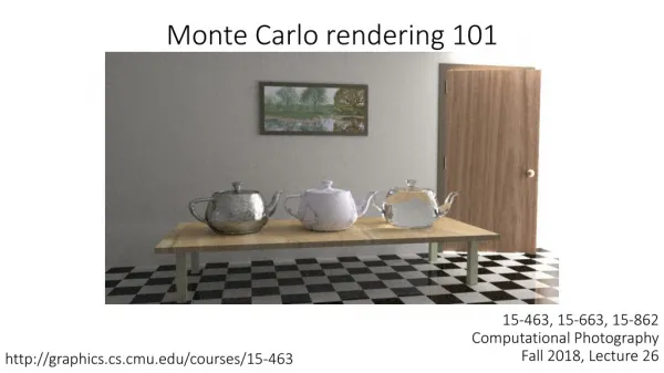
Monte Carlo Rendering
Monte Carlo Rendering. Central theme is sampling : Determine what happens at a set of discrete points, and extrapolate from there Central algorithm is ray tracing Rays from the eye or the light Theoretical basis is probability theory The study of random events. Random Variables.

Monte Carlo Rendering
E N D
Presentation Transcript
Monte Carlo Rendering • Central theme is sampling: • Determine what happens at a set of discrete points, and extrapolate from there • Central algorithm is ray tracing • Rays from the eye or the light • Theoretical basis is probability theory • The study of random events
Random Variables • A random variable, x • Takes values from some domain, • Has an associated probability density function, p(x) • A probability density function, p(x) • Is positive over the domain, • “Integrates” to 1 over :
Expected Value • The expected value of a random variable is defined as: • The expected value of a function is defined as:
Variance and Standard Deviation • The variance of a random variable is defined as: • The standard deviation of a random variable is defined as the square root of its variance:
Sampling • A process samples according to the distribution p(x) if it randomly chooses a value for x such that: • Weak Law of Large Numbers: If xi are independent samples from p(x), then:
Algorithms for Sampling • Psuedo-random number generators give independent samples from the uniform distribution on [0,1), p(x)=1 • Transformation method: take random samples from the uniform distribution and convert them to samples from another • Rejection sampling: sample from a different distribution, but reject some samples
Distribution Functions • Assume a density function f(y) defined on [a,b] • Define the probability distribution function, or cumulative distribution function, as: • Monotonically increasing function with F(a)=0 and F(b)=1
Transformation Method for 1D • Generate ziuniform on [0,1) • Compute • Then the xi are distributed according to f(x) • To apply, must be able to compute and invert distribution function F
Multi-Dimensional Transformation • Assume density function f(x,y) defined on [a,b][c,d] • Distribution function: • Sample xi according to: • Sample yiaccording to
Rejection Sampling • Say we wish to sample xi according to f(x) • Find a function g(x) such that g(x)>f(x) for all x in the domain • Geometric interpretation: generate sample under g, and accept if also under f • Transform a weighted uniform sample according to xi=G-1(z), and generate yiuniform on [0,g(xi)] • Keep the sample if yi<f(x), otherwise reject
Important Example • Consider uniformly sampling a point on a sphere • Uniformly means that the probability that the point is in a region depends only on the area of the region, not its location on the sphere • Generate points inside a cube [-1,1]x[-1,1]x[-1,1] • Reject if the point lies outside the sphere • Push accepted point onto surface • Fraction of pts accepted: /6 • Bad strategy in higher dimensions
Estimating Integrals • Say we wish to estimate • Write h=gf, where f is something you choose • If we sample xi according to f, then:
Standard Deviation of the Estimate • Expected error in the estimate after n samples is measured by the standard deviation of the estimate: • Note that error goes down with • This technique is called importance sampling • f should be as close as possible to g • Same principle for higher dimensional integrals
Example: Form Factor Integrals • We wish to estimate • Define • Sample from f by sampling xi uniformly on Pi and yi uniformly on Pj • Estimate is
Basic Ray Tracing • For each pixel in the image • Shoot a ray from the eye through the pixel, to determine what is seen through that pixel, and what its intensity is • Intensity takes contributions from: • Direct illumination (shadow rays, diffuse, Phong) • Reflected rays (recurse on reflected direction) • Transmitted rays (recurse of refraction direction)
Casting Rays • Given a ray, • Determine the first surface hit by the ray (intersection with lowest t) • Algorithms exist for most representations of surfaces, including splines, fractals, height fields, CSG, implicit surfaces… • Hence, algorithms based on ray tracing can be very general with respect to the geometry
Distributed Ray Tracing • Cook, Porter, Carpenter 1984 • Addresses the inability of ray tracing to capture: • non-ideal reflection/transmission • soft shadows • motion blur • depth of field • Basic idea: Cast more than one ray for each pixel, for each reflection, for each frame… • Rays are distributed, not the algorithm. Should probably be called distribution ray tracing.
Specific Cases • Sample several directions around the reflected direction to get non-ideal reflection, and specularities • Send multiple rays to area light sources to get soft shadows • Cast multiple rays per pixel, spread in time, to get motion blur • Cast multiple rays per pixel, through different lens paths, to get depth-of-field
What’s Good? What’s Bad? • Easy to implement - standard ray tracer plus simple sampling • Which L(D|S)*E paths does it get? • Which previous method could it be used with to good effect?