
Advanced Parallel Computing Algorithm: GPC
E N D
Presentation Transcript
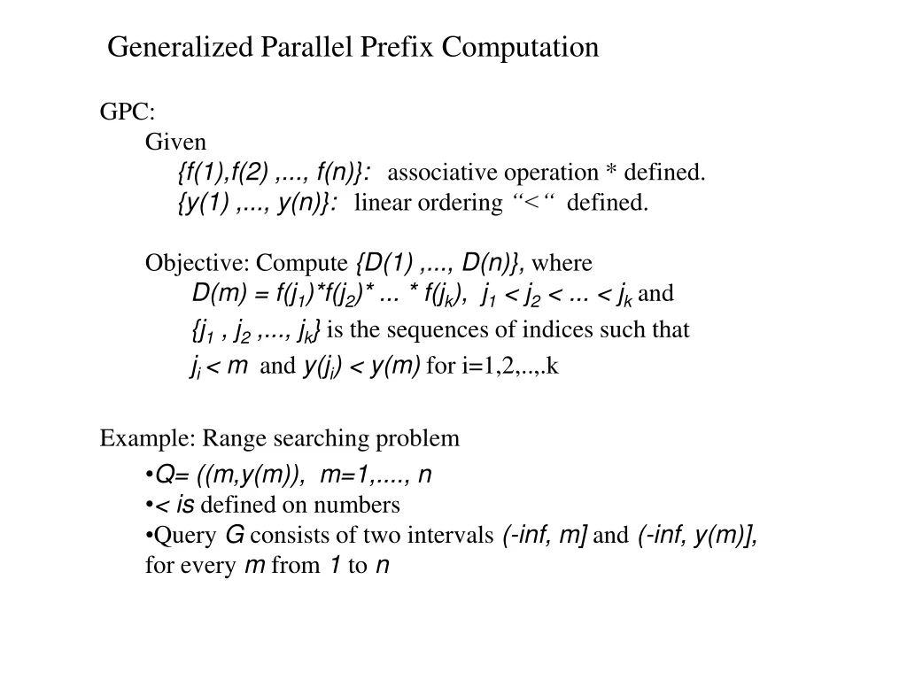
Generalized Parallel Prefix Computation • GPC: • Given • {f(1),f(2) ,..., f(n)}: associative operation * defined. • {y(1) ,..., y(n)}: linear ordering “<“ defined. • Objective: Compute {D(1) ,..., D(n)}, where • D(m) = f(j1)*f(j2)* ... * f(jk), j1 < j2 < ... < jk and • {j1 , j2 ,..., jk} is the sequences of indices such that • ji < m and y(ji) < y(m) for i=1,2,..,.k • Example: Range searching problem • Q= ((m,y(m)), m=1,...., n • < is defined on numbers • Query G consists of two intervals (-inf, m] and (-inf, y(m)], for every m from 1 to n
Generalized Parallel Prefix Computation GPC: Given {f(1),f(2) ,..., f(n)}: associative operation * defined. {y(1) ,..., y(n)}: linear ordering “<“ defined. Objective: Compute {D(1) ,..., D(n)}, where D(m) = f(j1)*f(j2)* ... * f(jk), j1 < j2 < ... < jk and {j1 , j2 ,..., jk} is the sequences of indices such that ji < m and y(ji) < y(m) for i=1,2,..,.k Example: Range searching problem • Q= ((m,y(m)), m=1,...., n • < is defined on numbers • Query G consists of two intervals (-, m] and (- , y(m)], for every m from 1 to n
Lower Bound of GPC If we can do GPC, then we can do sorting. Idea: Let {z(1), z(2),..., z(n) } all distinct. (i) f(j) = 1 for 1<= j <=n. (ii) y(j) = z(j), for 1<=i <=n. (iii) Compute D(m) (iv) y’(j) = z(n-j+1), for 1<=i <=n. (v) Compute D’(m) (vi) D(m) + D’(m): # of elements in Z smaller than z(m) Example: Z={4,5,3,7,1,6} D(m) = {0,1,0,3,0,4} D’(m) = {2,2,1,2,0,0} rank(m) = {2,3,1,5,0,4}
GPC Computation on PRAM • D(m,S): D(m) restricted on a sequence of indices S. That is, D(m,S) = f(j1)*f(j2)* ... * f(jk), where jiS and jisatisfies the conditions earlier (ji < m) • Y(S) : the sequence of elements y(j), jSin sorted order. • B(m,S):The position of y(m) in Y(S) • J(m,S) = {j1, j2, ... jr} be the subsequence of S satisfying y(ji)< y(m); For convenience, m is in J(m,S). • E(m,S) = f(j1)*f(j2)* ... * f(jr). y(i) m E(m,S) D(m,S) i
GPC Algorithm • Initially, S={1,...,n} • Partition S into two parts, L, and R • Apply algorithm recursively to L and R => Y(L), Y(R), D(l,L), D(r,R), E(l,L), E(r,R), B(l,L), B(r,R), for all l in L and r in R. • Compute Y(S) by merge Y(L) and Y(R). • Compute the rank B(m,S) in Y(S) for each r in R, gr: point in L with the largest y-value such that y(gr) < y(r), B(gr,L) = B(r,S) - B(r,R) => can find B(r,S) (How to find gr?) for each l in L. gl: The point in R with the largest y-value such that y(gl) < y(l), B(gl,L) = B(l,S) - B(l,L) => can find B(l,S) y(i) L R y(r) i
y(i) L R y(r) E(gr,L) D(r,R) i GPC Algorithm cont’ • Compute D and E as follows: D(l,S) = D(l,L) D(r,S) = E(gr,L) * D(r,R) E(l,S) = E(l,L) * E(gl,R) E(r,S) = E(gr,L) * E(r,R) y(i) R L 4 D(6,S) = E(2,L) * D(6,R) = f(1)*f(2)*f(3)*f(5) 7 6 y(r) 2 1 D(r,R) 8 5 3 i
Complexity • Similar to tree Computation • Depth of recursion log2n • Merging L and R into S • points of L, R sorted in y value • Points in S should be also sorted in y value • Then computinggris trivial • How to merge L and R in constant time?
Pipelined Merging of Two sorted list in a constant time(Cole’s Algorithm) • Leaves contain the value • Internal nodes merge at each time by updating the values • Lv: the sequence of values of descendants of v • Qv(j): At time j, a sorted sequence v has. An increasing subsequence of Lv When Qv(j) = Lv, then node v is complete. • All leaf nodes are complete. • At step j+1, if v’s parent is not complete at j-th step, it sends Rv(j) and Qv(j) to its parent. • Qv(j) = merge Rw(j) and Rz(j), where w and z are children of v • How to compute R? If w is not complete at j-1 step, Rw(j) consists of every 4-th elements of Qw(j-1). If w is complete after j step, (i) Rw(j+1) consists of every 4-th elements of Qw(j) (ii) Rw(j+2) consists of every 2nd elements of Qw(j) (iii) Rw(j+3) = Qw(j) • If w and z becomes complete at the j-th step, then v becomes complete at j+3 step • => total complexity 3logn • How to merge Rw(j) and Rz(j) in constant time?
Merging two samples in constant time • Two sequences S and T. • Predecessor of x in S: the largest element T smaller than x. • Example: S={1,3,4,9}, T={2,5,6,7} pred(3) = 2, pred(4) = 2, pred(5) = 4. • If each element of S and T know the position of its pred in T and S, => S and T can be merged in constant time using |S| + |T| PEs. • How to find the pred of Rw(j) and Rz(j) ? => Inductively. 1.Rw(j-1) and Rz(j-1) know their predecessors, and two sequence merged to Qv(j-1) . 2. each element in Rw(j-1) finds its pred in Qw(j-1) in constant time and its pred in Rw(j) in constant time. Note that no more than 4 elements of Rw(j-1) have the same pred in Rw(j) Each element in Rw(j) finds its pred in Rw(j-1) 3. Same for Rz. 4. With these pred knowledge, Rw(j) can determine their pred in Rz(j) in cons time.