PC-HYSPLIT WORKSHOP
PC-HYSPLIT WORKSHOP. National Oceanic and Atmospheric Administration. Air Resources Laboratory. Spring 2008. Workshop Agenda. 2. Model History. Version 1.0 - 1979 rawinsonde data with day/night (on/off) mixing 2.0 - 1983 rawinsonde data with continuous vertical diffusivity


PC-HYSPLIT WORKSHOP
E N D
Presentation Transcript
PC-HYSPLIT WORKSHOP National Oceanic and Atmospheric Administration Air Resources Laboratory Spring 2008
Workshop Agenda 2 PC-HYSPLIT WORKSHOP
Model History Version 1.0 - 1979 rawinsonde data with day/night (on/off) mixing 2.0 - 1983 rawinsonde data with continuous vertical diffusivity 3.0 - 1987 model gridded fields with surface layer interpolation 4.0 - 1996 multiple meteorological fields and combined particle-puff (NOAA Technical Memo ERL ARL-224) 4.0 - 8/1998 - switch from NCAR to PostScript graphics for PC 4.1 - 7/1999 - isotropic turbulence for short-range simulations 4.2 - 12/1999 - terrain compression of sigma and use of polynomial 4.3 - 3/2000 - revised vertical auto-correlation for dispersion 4.4 - 4/2001 - dynamic array allocation and support of lat-lon grids 4.5 - 9/2002 - ensemble, matrix, and source attribution options 4.6 - 6/2003 - non-homogeneous turbulence correction and dust storm 4.7 - 1/2004 - velocity variance, TKE, new short-range equations 4.8 - 2006 - CMAQ compatibility, expanded ensemble options, plume rise, Google Earth, trajectory clustering, staggered grids 3 PC-HYSPLIT WORKSHOP
Model Features • Predictor-corrector advection scheme • Linear spatial & temporal interpolation of meteorology from external sources • Vertical mixing based upon SL similarity, BL Ri, or TKE • Horizontal mixing based upon velocity deformation, SL similarity, or TKE • Puff and particle dispersion computed from velocity variances • Concentrations from particle-in-cell or top-hat/Gaussian distributions • Multiple simultaneous meteorology and/or concentration grids 4 PC-HYSPLIT WORKSHOP
Computational Methods Eulerian versus Lagrangian Eulerian Modeling Approach • Concentrations are computed at every grid cell interface due to diffusion and advection. • ∂C/∂t = [advection] + [diffusion] + [source] + [sinks] • Computationally intensive as each grid cell must be calculated even if pollutants are not advected into the cell. • Suitable for complex emission and non-linear chemical conversion scenarios. 5 PC-HYSPLIT WORKSHOP
Computational Methods Eulerian versus Lagrangian • Lagrangian Modeling Approach • Concentrations computed by summing the mass of each pollutant puff that is advected through the grid cell • dC/dt = [diffusion] + [source] + [sinks] • May require thousands of particles to adequately model pollutant dispersion • Most applicable to point source applications 6 PC-HYSPLIT WORKSHOP
Computational Methods Lagrangian Puff Model • Puff Model • Source is simulated by releasing pollutant puffs at regular intervals over the duration of the release • Each puff contains the appropriate fraction of the pollutant mass • A puff is advected according to the trajectory of its center position • The size of the puff (horizontal and vertically) expands in time to account for the dispersive nature of a turbulent atmosphere • Concentrations are calculated at specific points (or nodes on a grid) by assuming that the concentrations within the puff have a defined spatial distribution 7 PC-HYSPLIT WORKSHOP
Computational Methods Lagrangian Particle Model • Particle Model • Source is simulated by releasing many particles over the duration of the release • In addition to the mean advective motion, a random motion component is added to each particle at each step according to the atmospheric turbulence at that time • A cluster of particles released at the same point will expand in space and time simulating the dispersive nature of the atmosphere • Concentrations are calculated by summing the mass of all the particles in a grid cell • In a homogeneous environment the size of the puff (in terms of its standard deviation) at any particular time should correspond to the second moment of the particle positions 8 PC-HYSPLIT WORKSHOP
Trajectory versus Concentration Plumes • A puff following a single trajectory cannot properly model the growth of a pollutant cloud if the wind varies in space and time. • Single puffs must split into multiple puffs or the simulation must use many particles. • Three trajectories (10, 100, 200 m AGL) were started every 4hrs (below, left) to represent the boundary layer transport. Similarly, 2500 particles were released to simulate the air concentration plume (below, right). • Note that the patterns represented by both are similar. In this case, the upper level trajectories (green/blue) are to the south (right) of the lower level trajectories indicating shear is present in the vertical. 9 PC-HYSPLIT WORKSHOP
Trajectory versus Concentration Plumes Animation of particle transport from last example Animation (right) of the 2500 particles that produced the concentration pattern shown below. Note the higher level particles (blue) moving out ahead of the slower lower level particles (black) 10 PC-HYSPLIT WORKSHOP
Particle, Puff, & Hybrid Definitions: • Particle: A point mass of contaminant. A fixed number of particles are released and are moved by a wind having mean and random components. They never grow or split. • Puff: A fully 3-D cylindrical puff (below, left), having a defined concentration distribution in the vertical and horizontal. Puffs grow horizontally and vertically according to the dispersion rules for puffs, and split if they become too large. • Hybrid: A circular 2-D object (planar mass, having zero vertical depth), in which the horizontal contaminant has a “puff” distribution (below, right). There are a fixed number of these in the vertical because they function as particles in that dimension. In the horizontal, they grow according to the dispersion rules for puffs and split if they get too large. Illustration of how a single particle (Q0) splits due to vertical diffusion into two particles Q2 and Q3. Illustration of how a single particle with radius R splits due to horizontal diffusion into four particles (Q1, Q2, Q3 and Q4) each with radius R/2. 11 PC-HYSPLIT WORKSHOP
Code Installation The following optional, but highly suggested, programs should be installed prior to installing the registered version of HYSPLIT. The trial version already includes Tcl/Tk, Ghostscript, and Info-Zip and, therefore, do not need to be reinstalled prior to installing the registered version over top of the trial version. Install all programs in the default directories to make HYSPLIT installation easier. • Tcl/Tk - Although the model can also be run from a DOS window using a command line interface, it is easier for novice users to use the GUI menus provided with the installation. These GUI menus use the Tcl/Tk interpreter. • Get Tcl/Tk 8.4.14 • Tcl/Tk Website • Ghostscript/Ghostview - By default, HYSPLIT creates high-resolution, publication quality graphics in PostScript format. These can be printed directly on any PostScript printer or viewed on the standard PC display and printed on any printer (even non-Postscript) if Ghostscript has been installed. • Get Ghostscript 8.13 • Get Ghostview 4.6 • Ghostscript Website • ImageMagick - One feature of the GUI is the ability to convert the Postscript graphics output file to other graphical formats. This capability is enabled through the installation of ImageMagick, which requires the prior installation of Ghostscript. • Get ImageMagick 6.3 • ImageMagick Website 12 PC-HYSPLIT WORKSHOP
Code Installation The following optional programs are used to display the HYSPLIT output in a GIS format. In the past we recommended installing ESRI ArcExplorer to display shapefiles (ESRI GIS format), and Google Earth to display kml/kmz files. However, recently, ESRI released a new application called ArcGIS Explorer that is similar to Google Earth, and although not as powerful as Google Earth, it can display both ESRI shapefiles and kml/kmz files in one application without license issues (free). The option is up to you. Install all programs in the default directories to make HYSPLIT installation easier. • ESRI ArcExplorer - a free GIS application to overlay HYSPLIT output with other GIS layers. ESRI no longer makes version 2.0.800 available on its website, however ArcExplorer 9.2 Java Edition has been tested and does work with HYSPLIT shapefiles. This training uses version 2.0.800. • Get ESRI ArcExplorer Version 2.0.800 • ESRI Website • Info-ZIP - used to compress kml files into kmz files for use in Google Earth and ESRI ArcGIS. • Info-ZIP website • ESRI ArcGIS - a free GIS application to overlay HYSPLIT output with other GIS layers. Similar to Google Earth, it can display both shapefiles and kml/kmz. • ESRI ArcGIS website • Google Earth - Graphical output from the trajectory and concentration programs can be exported into a compressed kml file (*.kmz) for use in Google Earth; a software package to display geo-referenced information in 3-dimensions. Make sure to read the licensing requirements before installing. • Google Earth website 13 PC-HYSPLIT WORKSHOP
Code Installation HYSPLIT self-installing executables Two versions of PC HYSPLIT are available and can be downloaded from the HYSPLIT website. (An Apple version is also available on the website, however this workshop will use the PC version). It is recommended that HYSPLIT be installed in the C:\hysplit4 directory, however it can be installed in other locations. This document will assume HYSPLIT is installed in the C:\hysplit4 directory. • setup48U.exe - (61 Mb) – trial version, does not support forecast data, no registration required • setup48R.exe - (21 Mb) – registered version, requires web site registration to download The following sub-directories will be installed with a proper installation of HYSPLIT: arcview – information on ESRI shapefiles bdyfiles – surface height, land-use, and roughness length files browser – custom tcl scripts to support the GUI help browser interface cluster – scripts and files to create trajectory cluster analysis concmdl – scripts and files to automate and customize concentration simulations csource – dll files required for the particle viewer & editor data2arl – programs to convert meteorological data to the HYSPLIT format document – most recent version of the technical documents and User’s Guide exec – all executables can be found in this directory gisprog – programs to convert text files to shapefiles grads – source code to convert HYSPLIT output and meteorological data to grads graphics – map backgrounds and map customization files guicode – tcl scripts required to run the GUI html – help files metdata – sample meteorological data file and program to read the data source – subroutines to compile the meteorological data conversion programs trajmdl – sample scripts and files to customize trajectory simulations cluster – scripts and files to create trajectory cluster analysis uninstall – programs to uninstall HYSPLIT utilities – graphical display utilities vis5d – scripts and files to create VIS5D output working – output written here; sample CONTROL files 14 PC-HYSPLIT WORKSHOP
Workshop Meteorology A set of meteorological data files were saved from the 1200 UTC cycle on December 19, 2005 for use in the workshop examples. These files can be downloaded to any directory, however it will be easier to find them if they reside in the hysplit4/working directory. The files can be downloaded from: • ftp://www.arl.noaa.gov/pub/archives/workshop Meteorological Data Files Map Background Files GFSFLL - Global Forecast on latitude/longitude grid countymap - county borders GFSFNH - Global Forecast on Northern polar stereographic grid floridamap - high-resolution Florida map GFSXFLL - Extended-range Global Forecast on lat/lon grid GFSLRFLL - Long-range Global Forecast on lat/lon grid FNLDUST.bin - Global Analysis for dust simulation NAMF12 - North American Mesoscale forecast on 12 km grid NAMF40 - North American Mesoscale forecast on 40 km grid RUC - Rapid Update Cycle forecast on 20 km grid MM5NA15 - AFWA MM5 over North America on a 15 km grid MM5NA45 - AFWA MM5 over North America on a 45 km grid ngm.dec95.002 - Nested Grid Model archive from December 1995 ngm.jan96.001 - Nested Grid Model archive from January 1996 ngm.jan96.002 - Nested Grid Model archive from January 1996 edas.aug07.001 - EDAS archive on 40 km grid 15 PC-HYSPLIT WORKSHOP
Model Operation Requirements A trajectory or concentration simulation only requires one file called CONTROL, which defines various model parameters and other input and output files. An optional file called SETUP.CFG may be present to define more advanced simulation features. The Graphical User Interface (GUI) provides a user-friendly way to create these files, set any other command line options that some of the post-processing graphics programs may require, and run HYSPLIT and associated programs. Alternatively, the CONTROL and SETUP.CFG files can be created with any text editor, such as Notepad, and then HYSPLIT and its associated programs can be run from the DOS command line. Starting the model from the GUI After a successful install, the PC desktop should contain a HYSPLIT shortcut with the following properties: Target: \hysplit4\guicode\hysplit4.tcl Start in: \hysplit4\working The HYSPLIT “Start in” directory contains sample CONTROL files that can be used for initial guidance to set up more complex simulations. These can be loaded into the GUI from the Retrieve menu tab under the Trajectory Setup or Concentration Setup menus. Examples include: • sample_conc - concentration simulation example from users guide • sample_traj - trajectory simulation example from users guide • back_conc - backward dispersion simulation for concentration • back_traj - backward trajectory simulation 16 PC-HYSPLIT WORKSHOP
Example Trajectory • Start the model by double clicking the HYSPLIT icon on the desktop. • Click on the green Menu button at the bottom of the first screen. • Click on the Trajectory menu tab and choose Trajectory Setup. • Click on the Retrieve button at the bottom of the menu. • Click the Browse button and find the file sample_traj in the working directory. • Click OK. • Click Save to save the configuration settings. • Click on the Trajectory menu tab and choose Run Standard Model. (Note: if a menu pops up says that a SETUP.CFG namelist file was found, choose Delete and Run) • When the model is complete (Complete Hysplit is shown), click on the Exit button. • Click on the Trajectory menu tab and choose Display Options and then Trajectory. • Click on the Execute Display button to display the trajectory in the GSview viewer. (Note: if your GSview is not registered, just click the Ok button.) • The resulting 3 trajectories should be identical to those shown to the right. More details on the trajectory model configuration will be given later. Follow these steps to run the sample trajectory case provided with the default installation of PC HYSPLIT 17 PC-HYSPLIT WORKSHOP
Example Concentration • Start the model by double clicking the HYSPLIT icon on the desktop. • Click on the green Menu button at the bottom of the first screen. • Click on the Concentration menu tab and choose Concentration Setup. • Click on the Retrieve button at the bottom of the menu. • Click the Browse button and find the file sample_conc in the working directory. • Click OK. • Click Save to save the configuration settings. • Click on the Concentration menu tab and choose Run Standard Model. (Note: if a menu pops up says that a SETUP.CFG namelist file was found, choose Delete and Run) • When the model is complete (Complete Hysplit is shown), click on the Exit button. • Click on the Concentration menu tab and choose Display Options and then Concentration. • Click on the Execute Display button to display the trajectory in the GSview viewer. (Note: if your GSview is not registered, just click the Ok button.) • The resulting concentration pattern should be identical to the one shown to the right. More details on the concentration model configuration will be given later. Follow these steps to run the sample concentration case provided with the default installation of PC HYSPLIT 18 PC-HYSPLIT WORKSHOP
Updating HYSPLIT Scan for Updates • A recent feature was added to the Advanced menu called Scan for Updates. • Choosing Check for Updates will check the dates of your executables and scripts with those on the ARL server, and if more recent ones are available you will be prompted to replace each with the update. • Replaced executables and scripts are placed in the updates folder and may be reversed if needed with the Reverse Updates option. • Once a significant number of updates are made, a new version will be posted to the website and must be downloaded and installed manually. • Only updates to the same version are permitted.
Errors Occasionally, the HYSPLIT GUI’s may become confused if the user enters information and then cancels those inputs prior to running the model. If this occurs, or if any problems prevent the model from producing expected results, exit the model GUI and restart. PC-HYSPLIT WORKSHOP