Forecasting smoke and dust using HYSPLIT
130 likes | 344 Views
Forecasting smoke and dust using HYSPLIT. Smoke Forecast System. Experimental testing phase began March 28, 2006 Run daily at NCEP using the 6Z cycle to produce a 24-hr analysis and a 48-hr forecast. Computational Cycle. Daily Procedure.

Forecasting smoke and dust using HYSPLIT
E N D
Presentation Transcript
Smoke Forecast System • Experimental testing phase began March 28, 2006 • Run daily at NCEP using the 6Z cycle to produce a 24-hr analysis and a 48-hr forecast • Computational Cycle • Daily Procedure • Satellite detection of fire location and heat released • Calculation of emissions • HYSPLIT run • Statistics calculation • Web distribution All smoke particles and continuous fires initialize the next day’s calculation
The smoke outlines are produced manually, primarily utilizing animated visible band satellite imagery. The locations of fires that are producing smoke emissions that can be detected in the satellite imagery are incorporated into a special HMS file that only denotes fires that are producing smoke emissions. These fire locations are used as input to the HYSPLIT model. Hazard Mapping System
Emissions • Fire locations from Hazard Mapping System Fire and Smoke Product (http://www.ssd.noaa.gov/PS/FIRE/hms.html) • The fire position data representing individual pixel hot-spots that correspond to visible smoke are aggregated on a 20 km resolution grid. • Each fire location pixel is assumed to represent one km2 and 10% of that area is assumed to be burning at any one time. • PM2.5 emission rate is estimated from the USFS Blue Sky (http://www.airfire.org/bluesky) emission algorithm, which includes a fuel type data base and consumption and emissions models
HYSPLIT Mass distribution: • Horizontal: Top hat • Vertical: 3D Particle • Number of lagrangian particles per hour: 500 • Produces surface to 100 m and surface to 5000 m 1-hr average PM2.5 concentrations on a 15-km resolution grid • Meteorology: WRF-NMM (AQF version) 12 km and GFS meteorology (outside the WRF-NMM domain) 1 degree. • Release height: assumed to be equal to the final buoyant plume rise height as computed using Briggs (1969), implying that the final rise is a function of the estimated fire heat release rate, the atmospheric stability, and the wind speed. • Smoke particles are assumed to have a diameter of 0.8 mm with a density of 2 g/cc • Wet removal is much more effective than dry deposition and smoke particles in grid cells that have reported precipitation may deposit as much as 90% of their mass within a few hours
Dust forecasting system • PM10 originated from northern Africa. • Meteorology: GFS (Global Forecasting System) model 50x50 km • Daily runs HYSPLIT (forecast 24 hours) • Output and postprocessing • Web posting
Dust emissions • Emisions based on desert land use (spatial reolution 1x1 degree) • F = 0.01 u*4, Westphal et al. (1987) • Dust emissions only occur during dry days when the friction velocity exceeds the threshold value (0.28 m/s for an active sand sheet). • The maximum flux permitted is 1 mg m-2 s-1.
HYSPLIT settings description • Mass distribution: • Horizontal: Top hat • Vertical: 3D Particle • Number of lagrangian particles per hour: variable • Produces surface to 100 m and surface to 5000 m 1-hr average PM10 concentrations on a 100-km resolution grid • Wet removal is much more effective than dry deposition and dust particles in grid cells that have reported precipitation may deposit as much as 90% of their mass within a few hours