HYSPLIT
HYSPLIT. Glenn Gehring, Technology Specialist III Tribal Air Monitoring Support Center g lenn.gehring@nau.edu 541-612-0899. Hy brid S ingle- P article L agrangian I ntegrated T rajectory model . WHAT??. What??. I think I’ll call it HYSPLIT. Who Provides it?.


HYSPLIT
E N D
Presentation Transcript
HYSPLIT Glenn Gehring, Technology Specialist III Tribal Air Monitoring Support Center glenn.gehring@nau.edu 541-612-0899
Hybrid Single-Particle Lagrangian Integrated Trajectory model WHAT??
What?? I think I’ll call it HYSPLIT
Who Provides it? • The Air Resources Laboratory (ARL) provides products related to atmospheric dispersion and air quality including the HYSPLIT model • ARL was mandated by Congress shortly after WWII to address concerns about pollution transport (nuclear fallout was among the initial concerns) • ARL is now within the National Oceanic and Atmospheric Administration (NOAA), which also houses the National Weather Service
What HYSPLIT Does • HYSPLIT is a modeling tool used for computing both wind trajectories in three dimensions and complex pollutant dispersion, as well as deposition patterns • It can be used on-line or downloaded and used on your computer • It can provide short term forecasts for pollutant dispersion, or wind trajectories, using National Weather Service forecast meteorological data • It can help us predict air quality and explore existing pollution episodes in near-real-time, as well as increase our understanding of past pollution episodes
Why Do We Use it? • To forecast smoke impacts from proscribed burns, wildfires or other releases • To assess what might be contributing to high pollutant concentrations observed on our monitors • To assess transport patterns • To assess day/night/seasonal differences • To assess monitoring networks • And, more But Mainly
To Find Out Where is it Going Proscribed burn
How Does it Work? Some day I’ll tell you. But right now my name isn’t Dr. Glenn and I don’t have a clue. Lets focus on how it is used. (Okay, maybe I have a clue but not detailed knowledge of the algorithms and such)
If You Want Details, They’re There http://www.arl.noaa.gov/ready/hysplit4.html
Ely Shoshone August 2002 Backward Trajectories (Michael Dalton’s work – monthly trajectory patterns)
Where did that high concentration come from? Vertical manifold Tubing for NOy Gas Analyzer Rack Toxics Flow Controller 316 Stainless Steel 1/8 inch tubing connects regulator to calibrator NOy Data Logger Continuous Particulate Sensor Unit NOx Calibrator SO2 Continuous Particulate Monitor Control Units Ozone CGA 660? Fitting must match bottle Zero Air Generator EPA Protocol Gas
First, Some ozone considerations Ozone is a Love/Hate thing We typically work here and ozone is bad here Source: http://spaceplace.nasa.gov/greenhouse/
Ozone “precursors,” such as NOx and VOCs are emitted from sources (can be natural sources) and in the presence of sunlight ozone can be generated Ozone can transport long distances (insert hot rod beetle emitting leaves)
Very important chemical reactions related to ozone: + Nitrogen oxide (NO) reacts with ozone ( driving ozone concentrations down and producing nitrogen dioxide () Nitrogen dioxide () can react with VOCs in the presence of sunlight and produce ozone The VOCs can be natural, such as a pine forest, or anthropogenic such as a wood pulp facility or gas station.
Backward trajectories from two ozone sites on 4/12/2003 Quapaw Nation 83ppb 8-hour ozone Coal fired power plant Coal fired power plant Cherokee Nation Stilwell Site 90ppb 8-hour ozone
Highest Passive Ozone (24-hour sample) NOx point sources in tons per year emissions
Quapaw Site on July 22, 2004 – Site’s highest 8-hr Ozone 93 ppb as an 8-hour average Notice NO is flat near zero. This indicates source is probably farther away (NOx is typically mostly NO out the stack). NOx = NO + NO2
Area 8-hr Ozone on July 22, 2004 Saint Louis Kansas City Quapaw Site Oklahoma City Tulsa Memphis Little Rock
July 22, 2004, 24-hour Backward Trajectories (NOAA Air Resource Laboratory HYSPLIT Model) proportional NOx point source emissions – 2002 EI Quapaw Site
Oologah Power Plant 48-hr dispersion (NOAA Air Resource Laboratory HYSPLIT Model) Quapaw Site
GRDA Power Plant 48-hr dispersion (NOAA Air Resource Laboratory HYSPLIT Model) Quapaw Site
Muskogee Power Plant 48-hr dispersion (NOAA Air Resource Laboratory HYSPLIT Model) Quapaw Site
Combined 48-hr dispersion (NOAA Air Resource Laboratory HYSPLIT Model) Quapaw Site
Forward Trajectory from 3 Coal-Fired Power Plants on July 22, 2004 (only includes endpoints that are less than 10 meters AGL)
Forward Trajectory from 3 Coal-Fired Power Plants on July 22, 2004 (only includes endpoints that are less than 20 meters AGL)
NE Oklahoma Coal-Fired Power Plant NOx EmissionsSource: EPA AirData (1999 EI) Most Relevant Winds for Ozone Tulsa Ozone Season Wind Rose, Lines Indicate the Direction the Wind Came FROM, and Colors Indicate Wind Speed (1984-1992, March 1 to October 31, from 8 AM to 6 PM) What if you live here? N E W 2003 Ozone Monitoring Locations (Red Dots) S 26.5% of Oklahoma facility NOx emissions are from Muskogee, Mayes and Rogers Counties (1999) 22.9% of Oklahoma facility NOx emissions are from three NE Oklahoma coal-fired power plants (1999)
Beside each option there is a “Help” button. Please use it. The met database and location (lat long) are chosen in previous screens In general, a smaller resolution dataset is better (12km is better than 40 km) Choose forward or backward Date/Time is UTC (same as Greenwich Mean Time) and NOT local time Set total run time to 24 hours, or more in some instances In a 8-hour ozone BT example you might want to set the UTC time to the end of the 8-hour concentration (remember to convert time), then have it start a new trajectory every hour and stop after 8 trajectories. It will then make a trajectory for each hour in the 8-hour ozone average. You can start the height of a backward trajectory from the monitor height, say 4-meters agl. For a forward trajectory from a point source you would set the height slightly above the sources stack, if it has one. Most of these settings can stay at their default settings Decide if you want a GIS shapefile, and/or a Google Earth file. The trajectory endpoints file will still be there. If you are using the endpoints file, you can have it dump meteorological data such as mixing height, temp, solar radiation, etc., along the trajectory path for additional analysis. Save the endpoints file as a text file from your browser
Backward trajectories Elevations of trajectories
Open Text File in Excel and Modify Then create feature class in GIS software
GIS for Air Quality (a TAMS/ITEP Course) Anyone can learn to use HYSPLIT – Just start And, feel free to contact me if you want assistance