Bode Plot
Bode Plot. Frequency Response Methods. Outline. What is frequency response Frequency Response Plots Bode and Nyquist (Polar) Rules for Constructing Bode Plot. What is frequency response. An important alternative approach to system analysis and design is the frequency response method.

Bode Plot
E N D
Presentation Transcript
Bode Plot Frequency Response Methods
Outline • What is frequency response • Frequency Response Plots Bode and Nyquist (Polar) • Rules for Constructing Bode Plot
What is frequency response An important alternative approach to system analysis and design is the frequency response method. The frequency response of a system is defined as the steady-state response of the system to a sinusoidal input signal. We will investigate the steady-state response of the system to the sinusoidal input as the frequency varies.
Advantages of the frequency response method • The sinusoidal input signal for various ranges of frequency and amplitude is readily available. • It is the most reliable and uncomplicated method for the experimental analysis of a system. • Control of system bandwidth. • The TF describing the sinusoidal steady-state behaviour of the system is easily obtained by replacing s with jω in the system TF.
Frequency response plots • Polar plot The TF G(s) can be described in the frequency domain by The above equation is used for the polar plot representation of the frequency response in the polar plane. polar plane Alternatively, the TF G(jω) can be represented by
Frequency response plots (cont’d) Example – polar plot Consider a simple RC circuit. The TF of the system is The sinusoidal steady-state TF is The polar plot is obtained from polar plot To draw the polar plot, R(ω) and X(ω) at typical frequencies, e.g., ω=0, ∞, are to be determined.
Frequency response plots (cont’d) Limitations of polar plots: • The addition of poles and zeros requires the recalculation of the frequency response. • The effect of individual poles and zeros is not indicated. A more widely used graphical tool to plot frequency response is the Bode diagram. • Bode plot The TF in the frequency domain can be written as For a Bode diagram, we normally use Magnitude versus ω and phase versus ωare plotted separately.
Bode diagram Advantages of Bode plots: • Multiplication of magnitudes can be converted into addition by virtue of the definition of logarithmic gain. • Straight-line asymptotes are simple to be used for sketching an approximate log-magnitude curve. The use of a logarithmic scale for the frequency is a more judicious choice than a linear scale of frequency as this expands the low frequency range, which is more important in practical systems. An interval of two frequencies with a ratio equal to 10 is called a decade. The slope of the asymptotic line in the figure is -20dB/decade.
Rules for Constructing Bode Plot To draw Bode Plot there are four steps: 1.Rewrite the transfer function in proper form. 2.Separate the transfer function into its constituent parts. 3.Draw the Bode diagram for each part. 4.Draw the overall Bode diagram by adding up the results from part 3.
1.Rewrite the transfer function in proper form. • Make both the lowest order term in the numerator and denominator unity. Example 1:
2.Separate the transfer function into its constituent parts. • The next step is to split up the function into its constituent parts. There are seven types of parts: • A constant • Poles at the origin • Zeros at the origin • Real Poles • Real Zeros • Complex conjugate poles • Complex conjugate zeros
2.Separate the transfer function into its constituent parts. This function has a constant of 2, a zero at s=-10, and poles at s=-3 and s=-50. Example 2:
Magnitude Phase Slope= -20n db/dec -90n° 0 db wb Magnitude Phase Slope= +20n db/dec +90n° 0 db wb Draw Bode Plot Procedure
Phase 0° Magnitude 0 db Slope= -20n db/dec 0.1wb wb -90n° 10wb 10wb Magnitude Phase +90n° Slope= +20n db/dec 0.1wb 0 db wb 0° Draw Bode Plot Procedure
Phase 0° Magnitude 0 db Slope= -40n db/dec 0.1wb wb -180n° 10wb 10wb Magnitude Phase +180n° Slope= +40n db/dec 0.1wb 0 db wb 0° Draw Bode Plot Procedure
Bode Plot Procedure • The following example illustrates this procedure: 1.Rewrite the transfer function in proper form. 2.Separate the transfer function into its constituent parts.
Bode Plot Procedure 3.Draw the Bode diagram for each part.
Bode Plot Procedure 4.Draw the overall Bode diagram by adding up the results from part 3.
Check your AnsWer! • Step 2: Separate the transfer function into its constituent parts. • The transfer function has 2 components: • A constant of 3.3 • A pole at s= -30
Bode Plot Procedure Create the Phase Plot
Bode Plot Procedure The Phase plot compared to the computer generated plot then becomes:
Try This! Draw the Bode Diagram for the transfer function: REMEMBER the four steps: 1.Rewrite the transfer function in proper form. 2.Separate the transfer function into its constituent parts. 3.Draw the Bode diagram for each part. 4.Draw the overall Bode diagram by adding up the results from part 3.
Check your AnsWer! • Step 1: Rewrite the transfer function in proper form. • Make both the lowest order term in the numerator and denominator unity. The numerator is an order 0 polynomial, the denominator is order 1.
Check your AnsWer! • Step 3: Draw the Bode diagram for each part. • The constant is the cyan line (A quantity of 3.3 is equal to 10.4 dB). The phase is constant at 0 degrees. • The pole at 30 rad/sec is the blue line. It is 0 dB up to the break frequency, then drops off with a slope of -20 dB/dec. The phase is 0 degrees up to 1/10 the break frequency (3 rad/sec) then drops linearly down to -90 degrees at 10 times the break frequency (300 rad/sec). • Step 4: Draw the overall Bode diagram by adding up the results from step 3. • The overall asymptotic plot is the translucent pink line, the exact response is the black line.
The loop gain Transfer function L(s) The gain margin is defined as the multiplicative amount that the magnitude of L(s) can be increased before the closed loop system goes unstable Phase margin is defined as the amount of additional phase lag that can be associated with L(s) before the closed-loop system goes unstable Definition of Gain Margin and Phase Margin
Summary • Root locus analysis • Frequency response plots • Nyquist (nyquist) • Bode (bode) • Gain Margin • Phase Margin