Download

1 / 69
690 likes | 711 Views
Delve into Ordinary Least Squares regression theory, model assumptions, diagnostics, & advanced topics like limited dependent variables. Unpack history, terminologies, & advantages of linear regression in this comprehensive course.

E N D
Ordinaryleastsquares regressionnicholascharronassociate prof. Dept. ofpolitical science
Section Outline Day 1: overviewof OLS regression (Wooldridge, chap. 1-4). Intro to OLS, bivariate regression, significance, model diagnostics (review for many of you ) Day 2 (25 jan): assumptions of OLS regression, multivariate regression (Wooldridge, chap. 5-7) Day 3 (28 jan): alternative estimation, interaction models (Wooldridge, chap. 8-9 + Brambor et al article) Nexttopic (withme): Limiteddependentvariables – nextweek!
Section Goals • Course assumesyouhaveabackground, so this is ’advanced’, butapplied: Goals: • To understand the basicideas and formulasbehindlinear regression • Be abletocalculate (by hand) simple bivariate regression coefficient • Workingwith ’real’ data, applyknowledge, perform regression & interpret results, compareeffects of variables in multiple regression • Understand the basicasumptions of OLS estimation, how to check for violations, and what to do. • What to do when X and Y relationship are not directlylinear – interaction effect, variable transformation (logged, quadradicvariables for ex.) • Applyknowledge in STATA • Learnwithoutgettingtoobored
Introductions!-Name-Department-year as PhD student -whereyouare from (country/countries) -howmuchstatisiticshaveyouhad?-haveyouused STATA before?-a bit on your research topic?
Linear Regression: briefhistory Sir Francis Galton– interested in heredity, and testedideas in plants, ’regression towardmediocraty’, meaning in histime the median (nowknownmore as regression toward the mean ) Emphais on ’on average’ whatcanweexpect? - Hewas not a mathmaticianhowever(used median, interquartilerange) Karl Pearson (Galton’sbiographer) tookGalton’swork and developedseveral statistical measures Togetherwithprevious ’leastsquares’ method (Gauss 1812), regression analysiswasborn!
Simple statistical methods: cross tabulations, correlations • Usedwidely, especially in survey research, probablymany of youarefamiliarwith x-tabs& correlation • Whenwehave at leastoneCategoricalvariable– nominal or ordinal (difference?) • If we want to know how two variables related in terms of: strength, direction & effect, we can use various tests: • Nominal level – only strength (Cramer’s V) • Ordinal level – strength and direction (tau-b & tau-c, gamma) • Interval (ratio) level – strength, direction (and effect) (Pearson’s r, regression)
WHY DO WE USE LINEAR REGRESSION? • To test hypotheses about causal relationships for a continuous/ordinal outcome • To make predictions • The preferred method when your data is observational, &/or the statistical model has 2+ explanatory variables and you want to elaborate/control for in testing a causal relationship • Yet, the regression doesn’t necessarily express causal direction (why theory is important!) • So, always remember that correlation is not causation!
Keyadvantagesoflinear regression • Simplicity: a linear relationship is the most simple, non-trivial relationship. Plus, mostpeoplecaneven do the math by hand (as opposedtootherestimationtechniquesyou’llsee in thiscourse and elsewhere..) • Flexability: evenif the relationship between X and Y is not reallylinear, the variablescan be transformed (more later) • Interprebility: we get strength, direction &effect in a simple easy to understand package
Someessentialterminology – & ask ifunclear!! Regression: the mean of the outcomevariable (Y) as a function of 1+ independent variables (X) Regression Model: explainingY’s in the ’real world’ is verycomplicated. A model is ourAPPROXIMATION (simplification) ofour relationship Simple (bivariate) regression model Y: the dependentVariable X: the independent variable : the interceptor ’constant’ (in otherwords??), alsonotated as (alpha) sometimes : the slope – e.g. the expectedchange in Y given a oneunitchange in X ’s arecalled ’coefficients’
More terminology • Dependentvariable(Y): akaexplainedvariable, outcomevariable • Independent Variable(X): aka. Explanitoryvariable, controlvariable, sometimeseven ’parameter’, or ’constraint’ Two types of models broadly speaking: 1. Deterministic model: • Y=a+bx (the equation of a straight line) 2. Probabilistic model (e.g. what we are most interested in..): • Y=a+bx+e – (where we allow for error)
*Calculation of the slope (range of Y over range of X): *Calculation of intercept (for determinisitc models, just take any Y value & subtract βX): ex. α = 50 – (2 15) = 20, or α = 80 – (4 15) = 20 The equation for the relationship: Y = α + βX = 20 + 15X A deterministic model: simple ex.
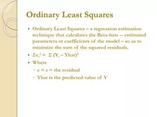
Evenmoreterminology • and, mostoften, we’redealingwith ’probabilistic’ models, so thesewords come upalot: Fittedvalues (’Y hat’): for any observation ’i’ ourmodel gives an expectedmean: Residual: is the error (howmuchourmodel is ’off’ the regression line) for obs ’i’ Where is normallywritten as Least Squares: ourmethodtofind the estimatesthatMINIMIZE the SUM of SQUARE RESIDUALS (SSE)
OLS- Regression Eachdotrepresents a respondent’sincome(Y) at age(X) Relationship betweenmonthly SEK income and age
OLS- Regression Relationship between income and age – shows strength, direction & effect, butcausality?
OLS- Regression Relationship betweenincome and age – *Diff between observed values and line is the error term = everything else that explains variation in Y but is not included in our model
Howtoestimate the coefficients? • We’ll go furtherthan Sir Galten & use the ’leastsquaresmethod’! To calculate the slopecoefficient () of X: the slopecoefficient is the covariancebetween X and Y over the varianceof X, or the rate of change of Yrelative to change in X And tocalculate the constant: Simplyspeaking, the constant is just the mean of Y minus the mean of X times
In classexcercise – Calculation of beta and alpha value in OLS by hand!
A cool property of leastsquaresestimation is that the regression linewillalways cross the mean of X and mean of Y • Now for everyvalueof X, wehave an expectedvalueof Y
compared to Pearson’s r • The effect in a linear regression = Correlation – Pearson’s r (-1 to 1) • Same numerator, but takes the variance of Y also in the denominator into account and ‘standardizes’ the variance w/ standard deviation of X and Y
Interpretation of Pearson’s r Source: wikipedia
Correlation and regression, cont. • Pearson’s r is standardized and varies between -1 (perfect neg. relationship) and 1 (perfect pos. relationship) 0 = no relationship, n is not taken into account • The regression coefficient () has no given minimum or maximum values and the interpretation of the coefficient depends on the range of the scale • Unlike the correlation r, the regression is used to predict values of one variable, given values of another variable • However, in significance testing (bivariate), the p-values will be approx. equal.
Objectives and goalsoflinear regression • Wewanttoknow the probability distribution of Y as a functionof X (or severalX’s) • Y is a straitline (e.g. linear) functionof X, plus somerandomnoise (error term) • Goal is tofind the ’best line’ that fits explains variation of Y with X • Important! The marginal effectof X on Y is assumedto be CONSTANT across all valuesof X. Whatdoesthismean??
Applied bivariate example • Data: QoG Basic, two variables from World Value Survey • Dependent variable (Y): Life happiness (1-4, lower=better) • Independent variable (X): State of health (1-5, lower=better) • Units of analysis: countries (aggregated from survey data ), 20 randomly selected Our Model: Y(Happiness) = α + β1(health) + e • H1: the healthier a country feels, the happier it is on average • Let’s Estimete of α and β1 based on our data! • Open filein STATA from GUL: health_happyex.dta
In classlabwork – alone or with partner • Go to GUL page under ’dokument’ & ’Charron OLS - open data file and producesummarystatistics of the 2 variables -what do yousee? (sum, tab, sum,d) • Check the Pearson’s rcorrelationcoefficient – what do youseehere? (pwcorr) • Produce a scatterplotwithhealth on the x-axis and happiness on y-axis (scatter) 4. Do a regression toestimateourmodel: Y(Happiness) = α + β1(health) + e (reg) & Interpret the regression table as best youcan: including the Beta, constant, and all other statistics thatyourecognize 5. What is the predictedmean of happines for a country with a mean in health of 2.3?
Somebasic statistics • Summary stats 2. Pairwisecorrelations (Pearson’s r)
3. Scatterplot w/line – in STATA:twoway(scatter happiness health) (lfit happiness health)
Observations • F-test of model sig. • R sq • Mean sq. error 4. the regression Coefficient (b) Constant (a) standard error t-test (of sig.) 95% interval ofconfidence
5. Some interpretation What is the predictedmean of happines for a country with a mean in health of 2.3?
Interpretation Y=.243 + .778(2.3) = 2.02 What is the predictedmean of happines for a country with a mean in health of 2.3? Answer: 2.02..
If youare still unsure, To do whatI’vedone in the slides, see the do.file: OLS d1 Charron.do
Ok, nowwhat?? • Ok great, but the calculation of beta and alphaare just simple math… • Now, wewanttoseehowmuchwecan INFER from this relationship – as we do not have ALL the observations (e.g. a ’universe’) withperfect data, weareonlymaking a ’probabilistic’ inference • A keytodoingthis is toevaluatehow ”off” ourmodelpredictionsare relative toactual observations in Y • Wecan do thisboth for ourmodel on whole and for individualcoefficients (both betas and alpha). We’ll start withcalculating the SUM of SQUARES • Twokeyquestions: • how ’sure’ areweofourestimates, e.g. significance, or probabilitythat the relationship wesee is not just ’whitenoise’ • Is this (OLS) actually the most valid estimationmethod?
Assumptions of OLS (more on this later!) OLS is fantastic if our data meets several assumptions, and before we make any inferences, we should always check: In order to make generalizable inferences: • The linear model is suitable • The conditional standard deviation is the same for all levels of X (homoskedasticity) • Error terms are normally distributed for all levels of X • There are no severe outliers • There is no autocorrelation • No multicollinearity • Our sample is representative of the population (random selection in case of survey for ex.)
Regression Inference In order to test several of our assumptions, we need to observe the residuals in our estimation These allow us to both check OLS assumptions AND provide significance testing Plotting the residuals against the explanatory (X) variable is helpful in checking these conditions because a residual plot magnifies patterns. This you should ALWAYS look at
Least squares: Sum of the squared error term – getting our error terms • A measure of how far the line is from the observations, is the sum of all errors: The smaller it is, the closer is the line to the observations (and thus, the better our model.) • In order to avoid positive and negative errors to cancel out in the calculation, we square them. Yi is the actual value & is our predicted value from our regression • The sum of all for observation i: The error term The Residualsumofsquares (RSS)
Back to our exercise: The typical deviation around the bar (ie the conditional standard deviation) mean square. D.f.=n- # of parameters
Getting our standard errors for beta = Where RSS= Residual Sum of Square, aka Sum of Squared Errors n=number of cases (in our example, n=20) K=number of parameters (in bivariate regression - intercept and b-coefficient = 2 The standard error (s.e.) tells us something about the average deviation between our observed values and our predicted values. The s.e. for a slope coefficient is then calculated as the square root of the RSS divided by the number of observations - the # of parameters (e.g. X’s + constant).
Getting our standard errors for b • The precision of β depends (among others) on the variation around the slope – i.e. how large the spread is around the line? • This spread, we have assumed constant for all levels of X, but how is it calculated? • See earlier: The sum of squared deviations of the line (RSS) is given by: • As we just saw, the typical deviation around the bar (ie the conditional standard deviation) is then given by:
Standard errors for β • βstandard error is then defined as the conditional standard error divided by the standard deviation of X (e.g. Sq. root of variance in X) Factors affecting the standard error of Beta: • The spread on the line σ - the smaller σ, the smaller the standard error • Sample size: n - the larger n, the smaller the standard error • The variation of X: - the greater the variation, the smaller the standard error
Back to our example (see excel sheet ‘Regression –health vs happiness’ for ‘by hand’ calculations..) Standard error of alpha Standard error of beta
Standard errors for β The standard errors can then be used forhypothesis testing. By dividing our slope-coefficients by their s.e.’s we receive their t-values. The t-value can then be used as a measure for statistical significance and allows us to calculate a p-value – evidence against the Ho Standard def: probability the model’s summary ≥ to the observed relationship assuming Ho is true Calcuations: Old school: one can consult a t-table where the degrees of freedom (the number of observations - 1) and your level of security (p<.10, .05 or .01 for ex.) decides whether your coefficient is significantly different from zero or not (t-table – can be found as appendices in books in statistics, like Woodbridge) New school: rely on statistical programs (like STATA, SPSS, R) H0: β1= 0 H1: β1≠ 0