Generalized Least Squares for Graph-Embeddable Problems

1. Generalized Least Squares for Graph-Embeddable Problems Giorgio Grisetti Special thanks to: Rainer Kuemmerle, Hauke Strasdat,Kurt Konolige,Cyrill Stachniss, Wolfram Burgard,

2. Least Squares • Find the minimum of a multivariate error function in this form • Usually addressed by standard methods like Gauss-Newton or Leveberg-Marquardt. • Many problems in robotics or computer-vision are reduced to least-squares optimization. SPD information matrix error function state vector

3. Least Squares on a Graph • Several problems like bundle-adjustment or SLAM result in an even more particular structure of the error function • The error vectors depend on pairs of state variables. • Thinking to the problem as a graph helps to exploit sparsity. • We can represent the problem as a graph: • The nodes of the graph represent state variables • An edge between two nodes represents the error function and the information matrix of a constraint involving the connected nodes.

4. Least Squares on a Graph • Several problems like bundle-adjustment or SLAM result in an even more particular structure of the error function • The error vectors depend on pairs of state variables. • We can represent the problem as a graph: • The nodes of the graph represent state variables • An edge between two nodes represents the error function and the information matrix of a constraint involving the connected nodes. • Thinking to the problem as a graph helps to exploit sparsity. edge vertices

5. Motivation • In this talk we present a general framework for least squares on a graph. • Our system offers performances comparable to those of ad-hoc approaches for SLAM or BA, while being compact and general • It is designed to be quickly and efficiently applied to new problems and it supports the most recent algorithms for solving sparse systems • It can take advantage of special structures of the graph, like the ones that occur in BA. • It will be released as an open-source C++ library and it will be part of ROS.

6. Example: Laser-based SLAM • SLAM = simultaneous localization and mapping • Estimate the robot’s poses and the map simultaneously • Use a graph to represent the problem • Every node in the graph corresponds to a pose of the robot during mapping • Every edge between two nodes corresponds to the spatial constraints between them • Goal: Find the configuration of the nodes that minimizes the error introduced by the constraints

7. Example: Laser-based SLAM • Goal: Find the arrangement of the nodes that satisfies the constraints best An initial configuration (KUKA production hall 22)

8. Example: Laser-based SLAM • Goal: Find the arrangement of the nodes that satisfies the constraints best An initial configuration Maximum likelihood configuration

9. Example: Laser-based SLAM • Goal: Find the arrangement of the nodes that satisfies the constraints best An initial configuration Maximum likelihood configuration

10. Example: Laser-based SLAM

11. Example: Vision SLAM

12. Example: Bundle Adjustment • Given a sequence of camera images taken from the same and a set of known point correspondences, • Find the optimal position of the cameras and the 3D location of the observed points in the world such that the reprojection error is minimized. Image courtesy of Noah Snavely

13. Example: Portable Scanner • <show DACUDA video>

14. Example Graphs • In SLAM • The nodes are the robot locations • An edge between two nodes is the relative motion between two robot positions that arises by matching the corresponding laser observations • In BA • The nodes are either camera positions or 3D points • An edge between a camera and a point is labeled with the image location of that 3D point. • The problem is entirely defined by specifying: • the domain the state variables (nodes), and • the error functions (edges).

15. Least Squares on a Graph • Some notation • Error function to minimize mean and informationmatrix of the observation observation of error between current state and observation edge

16. Iterative Solution • Linearize the error around the current solution x0 by fixing x and varying a small increment Δx • Thus the error terms in the neighborhood of the liearization become a quadratic form

17. Iterative Solution • Linearize the error around the current solution x0 by fixing x and varying a small increment Δx • Thus the error term in the neighborhood of the linearization becomes a quadratic form

18. Iterative Solution • …And the same happens to the global error function • The optimum of the quadratic form can be easily found by solving the linear system • The improved estimate is obtained by applying the perturbation to the previous guess

19. Iterative Solution • …And the same happens to the global error function • The optimum of the quadratic form can be found by solving the linear system • The improved estimate is obtained by applying the perturbation to the previous guess

20. Iterative Solution • …And the same happens to the global error function • The optimum of the quadratic form can be found by solving the linear system • The improved estimate is obtained by applying the perturbation to the previous guess

21. Jacobians and Sparsity • In error function eij of a constraint depends only on the two parameter blocks xi and xj • Thus the Jacobian will be 0 everywhere but in the columns of xi and xj. • This leads to a sparse pattern in the matrix H, that reflects the adjacency matrix of the graph.

22. Jacobians and Sparsity • In error function eij of a constraint depends only on the two parameter blocks xi and xj • Thus the Jacobian will be 0 everywhere but in the columns of xi and xj. • This leads to a sparse pattern in the matrix H, that reflects the adjacency matrix of the graph.

23. Consequences on the Structure Non zero only @ xi and xj

24. Consequences on the Structure Non zero only @ xi and xj Non zero on the main diagonal @ xi and xj

25. Consequences on the Structure Non zero only @ xi and xj Non zero on the main diagonal @ xi and xj .. and at the blocks ij,ji

26. Consequences on the Structure + + … + + … + +

27. Solution of the Linear System • Different structures benefit from different solvers • CHOLMOD • COLAMD • PCJ • … • In our framework the solution of the linear system is decoupled from the rest. • We provide drivers for the most common solvers, and you can easily integrate your own.

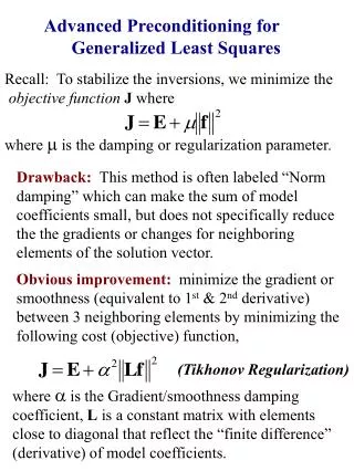
28. Special Structures • Special structures can be handled with ad-hoc solvers • Schur complement • Partial marginalizations • Approaches: • Decoupling the construction of the linearized system from the calculation of the Hessian. • Efficient implementation of the Schur complement. • Taking advantage of the features of the most recent CPUs (SSE, MMX, NEON), speed X4.

29. Overview

30. Overview Problem specific

31. Overview This comes for free (numerically computed). If you specify Jij analytically it gets faster

32. Overview Exploit the a-priori knowledge of the structure

33. Overview Choose your favorite linear solver

34. A Small Example: 2D Pose SLAM class VertexSE2 : public BaseVertex<3, SE2, 3, false> { public: virtual void oplus(double* update) { _estimate.translation() += Vector2d(update[0], update[1]); _estimate.rotation().angle() += update[2]; _estimate.rotation().angle() = normalize_theta(_estimate.rotation().angle()); } }; class EdgeSE2 : public BaseEdge<3, SE2, VertexSE2, VertexSE2, false> { public: void computeError() const { const VertexSE2* v1 = static_cast<const VertexSE2*>(_from); const VertexSE2* v2 = static_cast<const VertexSE2*>(_to); SE2 delta = _inverseMeasurement * (v1->estimate().inverse()*v2->estimate()); _error = delta.toVector(); } };

35. Experiments: SLAM

36. Experiments: BA

37. Experiments: Timings • Compared with ad-hoc systems: • Dellaert’s SAM • Konolige’s sSBA • Konolige’s SPA • Strasdat’s RobotVision

38. Experiments: Testing Different Parameterizations • Expmap better but more expensive

39. Experiments: Structure • In SLAM many poses, few landmarks: • Marginalizing the landmarks makes the reduced system more connected: harder to solve. • In BA many landmarks, few cameras: • Reducing the system makes sense.

40. Experiments: Linear Solvers • CSparse better than CHOLMOD on small systems, worse otherwise • PCG better when close to initial guess, bad otherwise: • OK in BA, OK for SLAM in open loop

41. Reasons to use this Framework • I need to solve a new graph optimization problem and I want to check if my error functions are correct. • Just define the domains of the parameters and the error functions. The Jacobians can be computed numerically by the system. • I wrote a new linear solver, I want to test it on a variety of problems. • Encapsulate your solver in a new driver and it can be use by all the problems that are already specified in the system (2D/3D SLAM with landmarks, bearing-only, poses, BA) • I think that my decomposition of the linear system that works well for problem X could also work for problem Y. • You can test it for free on all the problems, once you implement the appropriate driver. • I do not care about graph optimization. I just need to use this as a building block of my system.

42. Conclusions • Approach to generalized pose-graph optimization • Easy to adapt to new problems • Designed to be extended by using different system decompositions and different linear solvers. • Its performances are comparable to those of state-of-the art ad-hoc approaches, while being general. • Will be soon available as open-source (L-GPL v3)

43. Open Issues • How to construct a graph from raw data? • Is it possible to generalize? At which level? • How to reject wrong topologies [dynamics]? • Possibly abstract from raw data. • How to cope with weird initial guesses? • Very relevant in SLAM • Large Scale: • More efficient (bah)… • Dropping non-needed details (portions of the graph?). • Can’t know at the beginning what to neglect. • How to generalize on the abstraction/marginalization? • Should be SIMPLE!