Download
1 / 12
120 likes | 398 Views
Using Gravity Modeling to Understand the Subsurface Geology of the La Bajada Fault Zone. Hussam Busfar The University of Texas at Austin SAGE 2004. Objectives. Learn about gravity reduction and modeling process. Investigate the subsurface geology: Locate Fault(s) Detect density contrasts

E N D
Using Gravity Modeling to Understand the Subsurface Geology of the La Bajada Fault Zone Hussam Busfar The University of Texas at Austin SAGE 2004
Objectives • Learn about gravity reduction and modeling process. • Investigate the subsurface geology: • Locate Fault(s) • Detect density contrasts • Depth of units • Structure • Speculations and future improvement of data.
Data Collection • Instruments used: • La Coste – Romberg analog gravity meter • Scintrix Autograv meter. • Leica real-time differential GPS system: (elevation-horizontal coordinates) • 1 ft ≈ 0.3 m ≈ 0.06 mGal • Data were collected by current/previous SAGE students/faculty, USGS, and oil companies.
Study Area • Line of profile is ≈ 50 km. • First the data were corrected then least square fit method was used along the profile.
Processingthe data • The gravity data colleted in the field is influenced by many factors. • Raw data must be reduced • The corrections are: • Instrumental (meter) drift • Tidal effect • Latitude (pole ≈ 9.83 m/s2, equator ≈ 9.78 m/s2) • Free air • Bouguer • Terrain • For Bouguer/Terrain correction we assumed a density of 2.2g/cc and 2.67g/cc for elevations from 0-2 km and >2 km respectively.
Complete Bouguer Anomaly with Overlain Geology of Study Area
W E La Bajada fault • Inverse Model • Residual = Complete Bouguer – Regional anomaly • 3 density contrasts are plotted to fit the residual anomaly curve -0.35g/cc • -0.45g/cc -0.55g/cc • Each density contrast produces a different depth of sediments model • Fault dip >= 60° • Fault ≈ 17 km from W • Sediment thickness over fault? regional Bouguer residual
W E Another Fault? • Forward Model • Talwani Program • Depth to sediment model from the inverse model is used to produce the forward model. • Trial and error/horror! • Densities assumed from geology. • Fault: • dip >= 60 • ≈ 16 km from W • depth ≈ 1km
Complete Bouguer Anomaly with Overlain Geology of Study Area
W Faults E 0 2km Inverse Model ≈ 350m to W Forward Model ≈ 1.35km to W
Future Improvement of Study • Fill in gravity data • Constrain gravity models with well logs • Use other geophysical techniques to aid in gravity modeling
Conclusion • Gravity technique is relatively less expensive and fast. • Gives us some idea of the subsurface geology. • Gravity technique by itself gives us non-unique solutions • Much more useful if coupled with other geophysical techniques