Download
1 / 16
180 likes | 341 Views
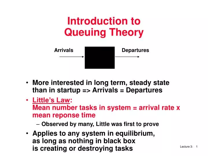
Introduction to Queuing Theory. More interested in long term, steady state than in startup => Arrivals = Departures Little’s Law : Mean number tasks in system = arrival rate x mean reponse time Observed by many, Little was first to prove

E N D
Introduction to Queuing Theory • More interested in long term, steady state than in startup => Arrivals = Departures • Little’s Law: Mean number tasks in system = arrival rate x mean reponse time • Observed by many, Little was first to prove • Applies to any system in equilibrium, as long as nothing in black box is creating or destroying tasks Arrivals Departures
System server Queue Proc IOC Device A Little Queuing Theory: Notation • Queuing models assume state of equilibrium: input rate = output rate • Notation: r average number of arriving customers/second ()Tser average time to service a task (traditionally m = 1/ Tser)u server utilization (0..1): u = r x m (or u= r / Tser )Tq average time/task in queue Tsys average time/task in system: Tsys = Tq + TserLser average number of tasks in service: Lser = r x Tser Lq average length of queue: Lq = r x Tq Lsys average length of system: Lsys = r x Tsys
Little’s Law Lengthsystem = rate x Timesystem (Mean number customers = arrival rate x mean service time) Lengthqueue = Arrival rate x Timequeue = r x Tq = Lq Lengthserver = Arrival rate x Timeserver = r x Tser = Lser
Example • Suppose an I/O system with a single disk gets about 10 I/O requests per second and the average time for a disk to service an I/O request is 50 ms. What is the utilization of the I/O system? • The service rate is 1/50ms = 20 I/O /sec • Server utilization = Arrival rate / Service rate = 10/20 = 0.5
Example • Suppose the average time to satisfy a disk request is 50 ms and the I/O system with many disks gets about 200 I/O requests per second. What is the mean number of I/O requests at the disk server? Lengthserver = Arrival rate X Timeserver (Lser = r x Tser) = 200x0.05 = 10 So there are 10 requests on average at the disk server
System server Queue Proc IOC Device A Little Queuing Theory • A single server queue: combination of a servicing facility that accommodates 1 customer at a time (server) + waiting area (queue): together called a system • Tsys = Lq x Tser + Mean time to complete service of tasks when new task arrives • Server spends a variable amount of time with customers; how do you characterize variability? • Distribution of a random variable: histogram? curve?
Random Variables • A variable is random if it takes one of a specified set of values with a specified probability • You cannot know exactly what its next value will be • But you do know the probability of all possible value • Usually characterized by Mean and Variance
System server Queue Proc IOC Device A Little Queuing Theory • Server spends a variable amount of time with customers • Weighted mean m1 = (f1 x T1 + f2 x T2 +...+ fn x Tn)/F (F=f1 + f2...) • variance = (f1 x T12 + f2 x T22 +...+ fn x Tn2)/F – m12 • Must keep track of unit of measure (100 ms2 vs. 0.1 s2 ) • Squared coefficient of variance: C = variance/m12 • Unitless measure (100 ms2 vs. 0.1 s2) • Exponential distribution C = 1: most short relative to average, few others long; 90% < 2.3 x average, 63% < average • Hypoexponential distributionC < 1: most close to average, C=0.5 => 90% < 2.0 x average, only 57% < average • Hyperexponential distributionC > 1: further from average C=2.0 => 90% < 2.8 x average, 69% < average Avg.
System server Queue Proc IOC Device A Little Queuing Theory: Variable Service Time • Server spends a variable amount of time with customers • Weighted mean m1 = (f1xT1 + f2xT2 +...+ fnXTn)/F (F=f1+f2+...) • Squared coefficient of variance C • Disk response times C ~= 1.5 (majority seeks < average) • Yet usually pick C = 1.0 for simplicity • Another useful value is average time must wait for server to complete task: m1(z) • Not just 1/2 x m1 because doesn’t capture variance • Can derive m1(z) = 1/2 x m1 x (1 + C) • No variance => C= 0 => m1(z) = 1/2 x m1
A Little Queuing Theory:Average Wait Time • Calculating average wait time in queue Tq • If something at server, it takes to complete on average m1(z) • Chance server is busy = u; average delay is u x m1(z) • All customers in line must complete; each avg Tser Tq = uxm1(z) + Lq x Ts er= 1/2 x ux Tser x (1 + C) + Lq x Ts er Tq = 1/2 x uxTs er x (1 + C) + r x Tq x Ts er Tq = 1/2 x uxTs er x (1 + C) + u x TqTqx (1 – u) = Ts er x u x (1 + C) /2Tq = Ts er x u x (1 + C) / (2 x (1 – u)) • Notation: r average number of arriving customers/secondTser average time to service a customeru server utilization (0..1): u = r x TserTq average time/customer in queueLq average length of queue:Lq= r x Tq
A Little Queuing Theory: M/G/1 and M/M/1 • Assumptions so far: • System in equilibrium • Time between two successive arrivals in line are random • Server can start on next customer immediately after prior finishes • No limit to the queue: works First-In-First-Out • Afterward, all customers in line must complete; each avg Tser • Described “memoryless” or Markovian request arrival (M for C=1 exponentially random), General service distribution (no restrictions), 1 server: M/G/1 queue • When Service times have C = 1, M/M/1 queueTq = Tser x u x (1 + C) /(2 x (1 – u)) = Tser x u / (1 – u) Tser average time to service a customeru server utilization (0..1): u = r x TserTq average time/customer in queue
A Little Queuing Theory: An Example • processor sends 10 x 8KB disk I/Os per second, requests & service exponentially distrib., avg. disk service = 20 ms • On average, how utilized is the disk? • What is the number of requests in the queue? • What is the average time spent in the queue? • What is the average response time for a disk request? • Notation: r average number of arriving customers/second = 10Tser average time to service a customer = 20 ms (0.02s)u server utilization (0..1): u = r x Tser= 10/s x .02s = 0.2Tq average time/customer in queue = Tser x u / (1 – u) = 20 x 0.2/(1-0.2) = 20 x 0.25 = 5 ms (0 .005s)Tsys average time/customer in system: Tsys =Tq +Tser= 25 msLq average length of queue:Lq= r x Tq= 10/s x .005s = 0.05 requests in queueLsys average # tasks in system: Lsys = r x Tsys = 10/s x .025s = 0.25
A Little Queuing Theory: Another Example • processor sends 20 x 8KB disk I/Os per sec, requests & service exponentially distrib., avg. disk service = 12 ms • On average, how utilized is the disk? • What is the number of requests in the queue? • What is the average time a spent in the queue? • What is the average response time for a disk request? • Notation: r average number of arriving customers/second= 20Tser average time to service a customer= 12 msu server utilization (0..1): u = r x Tser= /s x .s = Tq average time/customer in queue = Ts er x u / (1 – u) = x /() = x = msTsys average time/customer in system: Tsys =Tq +Tser= 16 msLq average length of queue:Lq= r x Tq= /s x s = requests in queueLsys average # tasks in system : Lsys = r x Tsys = /s xs =
A Little Queuing Theory: Another Example • processor sends 20 x 8KB disk I/Os per sec, requests & service exponentially distrib., avg. disk service = 12 ms • On average, how utilized is the disk? • What is the number of requests in the queue? • What is the average time a spent in the queue? • What is the average response time for a disk request? • Notation: r average number of arriving customers/second= 20Tser average time to service a customer= 12 msu server utilization (0..1): u = r x Tser= 20/s x .012s = 0.24Tq average time/customer in queue = Ts er x u / (1 – u) = 12 x 0.24/(1-0.24) = 12 x 0.32 = 3.8 msTsys average time/customer in system: Tsys =Tq +Tser= 15.8 msLq average length of queue:Lq= r x Tq= 20/s x .0038s = 0.076 requests in queueLsys average # tasks in system : Lsys = r x Tsys = 20/s x .016s = 0.32
A Little Queuing Theory:Yet Another Example • Suppose processor sends 10 x 8KB disk I/Os per second, squared coef. var.(C) = 1.5, avg. disk service time = 20 ms • On average, how utilized is the disk? • What is the number of requests in the queue? • What is the average time a spent in the queue? • What is the average response time for a disk request? • Notation: r average number of arriving customers/second= 10Tser average time to service a customer= 20 msu server utilization (0..1): u = r x Tser= 10/s x .02s = 0.2Tq average time/customer in queue = Tser x u x (1 + C) /(2 x (1 – u)) = 20 x 0.2(2.5)/2(1 – 0.2) = 20 x 0.32 = 6.25 msTsys average time/customer in system: Tsys = Tq +Tser= 26 msLq average length of queue:Lq= r x Tq= 10/s x .006s = 0.06 requests in queueLsys average # tasks in system :Lsys = r x Tsys = 10/s x .026s = 0.26