Download
1 / 40
400 likes | 533 Views
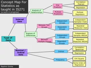
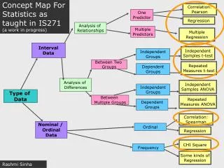
Concept Map For Statistics as taught in IS271 (a work in progress). Correlation: Pearson. One Predictor. Regression. Analysis of Relationships. Multiple Predictors. Multiple Regression. Interval Data. Independent Samples t-test. Independent Groups. Between Two Groups.

E N D
Concept Map For Statistics as taught in IS271 (a work in progress) Correlation: Pearson One Predictor Regression Analysis of Relationships Multiple Predictors Multiple Regression Interval Data Independent Samples t-test Independent Groups Between Two Groups Repeated Measures t-test Dependent Groups Analysis of Differences Independent Samples ANOVA Independent Groups Type of Data Between Multiple Groups Repeated Measures ANOVA Dependent Groups Correlation: Spearman Nominal / Ordinal Data Ordinal Regression CHI Square Frequency Some kinds of Regression Rashmi Sinha
Analysis of Variance or F test ANOVA is a technique for using differences between sample means to draw inferences about the presence or absence of differences between populations means. • The logic of ANOVA and calculation in SPSS • Magnitude of effect: eta squared, omega squared • Note: ANOVA is equivalent to t-test in case of two group situation
Logic of Analysis of Variance • Null hypothesis (Ho): Population means from different conditions are equal • m1 = m2 = m3 = m4 • Alternative hypothesis: H1 • Not all population means equal.
Lets visualize total amount of variance in an experiment Total Variance = Mean Square Total Between Group Differences (Mean Square Group) Error Variance (Individual Differences + Random Variance) Mean Square Error F ratio is a proportion of the MS group/MS Error. The larger the group differences, the bigger the F The larger the error variance, the smaller the F
Logic • Create a measure of variability among group means MSgroup • Create a measure of variability within groups MSerror • Form ratio of MSgroup /MSerror • Ratio approximately 1 if null true • Ratio significantly larger than 1 if null false • “approximately 1” can actually be as high as 2 or 3, but not much higher • Look up statistical tables to see if F ratio is significant for the specified degrees of freedom
Grand mean = 3.78 Hypothetical Data
Calculations • Start with Sum of Squares (SS) • We need: • SStotal • SSgroups • SSerror • Compute degrees of freedom (df ) • Compute mean squares and F Cont.
Degrees of Freedom (df ) • Number of “observations” free to vary • dftotal = N - 1 • N observations • dfgroups = g - 1 • g means • dferror = g (n - 1) • n observations in each group = n - 1 df • times g groups
When there are more than two groups • Significant F only shows that not all groups are equal • We want to know what groups are different. • Such procedures are designed to control familywise error rate. • Familywise error rate defined • Contrast with per comparison error rate
In case of multiple comparisons: Bonferroni adjustment • The more tests we run the more likely we are to make Type I error. • Good reason to hold down number of tests • Run t tests between pairs of groups, as usual • Hold down number of t tests • Reject if t exceeds critical value in Bonferroni table • Works by using a more strict level of significance for each comparison
Bonferroni t--cont. • Critical value of a for each test set at .05/c, where c = number of tests run • Assuming familywise a = .05 • e. g. with 3 tests, each t must be significant at .05/3 = .0167 level. • With computer printout, just make sure calculated probability < .05/c • Necessary table is in the book
Magnitude of Effect • Why you need to compute magnitude of effect indices • Eta squared (h2) • Easy to calculate • Somewhat biased on the high side • Percent of variation in the data that can be attributed to treatment differences
Magnitude of Effect--cont. • Omega squared (w2) • Much less biased than h2 • Not as intuitive • We adjust both numerator and denominator with MSerror • Formula on next slide
h2 and w2 for Foa, et al. • h2 = .18: 18% of variability in symptoms can be accounted for by treatment • w2 = .12: This is a less biased estimate, and note that it is 33% smaller.
Factorial Analysis of Variance • What is a factorial design? • Main effects • Interactions • Simple effects • Magnitude of effect
What is a Factorial • At least two independent variables • All combinations of each variable • Rows X Columns factorial • Cells 2 X 2 Factorial
Main effects • There are two factors in the experiment: Source of Review and Type of Product. • If you examine effect of Source of Review (ignoring Type of Product for the time being), you are looking at the main effect of Source of Review. • If we look at the effect of Type of Product, ignoring Source of Review, then you are looking at the main effect of Type of Product.
Simple effects • If you could restrict yourself to one level of one IV for the time being, and looking at the effect of the other IV within that level. • Effect of Source of Review at one level of Product Type (e.g. for one kind of Product), then that is a simple effect. • Effect of Product Type at one level of Source of Review (e.g. for one kind of Source, then that is a simple effect. Simple of Effect of Product Type at one level of Source of Review (I.e., one kind of Review Type, Expert Review)
Types of Interactions And this is when there are only two variables!
Magnitude of Effect F ratio is biased because it goes up with sample size. For a true estimate for the treatment effect size, use eta squared (the proportion of the treatment effect / total variance in the experiment). Eta Squared is a better estimate than F but it is still a biased estimate. A better index is Omega Squared.
Magnitude of Effect • Eta Squared • Interpretation • Omega squared • Less biased estimate k = number of levels for the effect in question
R2 is also often used. It is based on the sum of squares. For experiments use Omega Squared. For correlations use R squared. Value of R square is greater than omega squared. Cohen classified effects as Small Effect: .01 Medium Effect: .06 Large Effect: .15
Effects to be estimated • Differences due to instructions • Errors more in condition without instructions • Differences due to gender • Males appear higher than females • Interaction of video and gender • What is an interaction? • Do instructions effect males and females equally? Cont.
Estimated Effects--cont. • Error • average within-cell variance • Sum of squares and mean squares • Extension of the same concepts in the one-way
Calculations • Total sum of squares • Main effect sum of squares Cont.
Calculations--cont. • Interaction sum of squares • Calculate SScells and subtract SSV and SSG • SSerror = SStotal - SScells • or, MSerror can be found as average of cell variances
Degrees of Freedom • df for main effects = number of levels - 1 • df for interaction = product of dfmain effects • dferror = N - ab = N - # cells • dftotal = N - 1
Calculations for Data • SStotal requires raw data. • It is actually = 171.50 • SSvideo Cont.
Calculations--cont. • SSgender Cont.
Calculations--cont. • SScells • SSVXG = SScells - SSinstruction- SSgender= 171.375 - 105.125 - 66.125 = 0.125 Cont.
Calculations--cont. • MSerror = average of cell variances =(4.62 + 3.52 + 4.22 + 2.82)/4 =58.89/4 = 14.723 • Note that this is MSerror and not SSerror
Elaborate on Interactions • Diagrammed on next slide as line graph • Note parallelism of lines • Instruction differences did not depend on gender