Download
1 / 20
200 likes | 219 Views
Learn the logic, calculations in SPSS, effect size, and assumptions of ANOVA. Understand the F-ratio, degrees of freedom, and post-hoc tests for interpreting group differences.

E N D
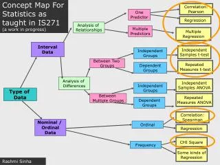
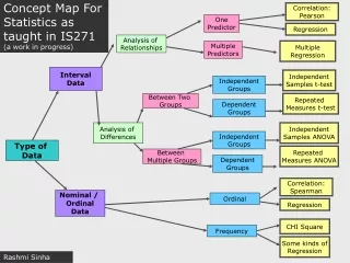
Concept Map For Statistics as taught in IS271 (a work in progress) Correlation: Pearson One Predictor Regression Analysis of Relationships Multiple Predictors Multiple Regression Interval Data Independent Samples t-test Independent Groups Between Two Groups Repeated Measures t-test Dependent Groups Analysis of Differences Independent Samples ANOVA Independent Groups Type of Data Repeated Measures ANOVA Between Multiple Groups Dependent Groups Correlation: Spearman Nominal / Ordinal Data Ordinal Regression CHI Square Frequency Some kinds of Regression Rashmi Sinha
Analysis of Variance or F test ANOVA is a technique for using differences between sample means to draw inferences about the presence or absence of differences between populations means. • The logic • Calculations in SPSS • Magnitude of effect: eta squared, omega squared
Assumptions of ANOVA • Assume: • Observations normally distributed within each population • Population variances are equal • Homogeneity of variance or homoscedasticity • Observations are independent
Assumptions--cont. • Analysis of variance is generally robust to first two • A robust test is one that is not greatly affected by violations of assumptions.
Logic of Analysis of Variance • Null hypothesis (Ho): Population means from different conditions are equal • m1 = m2 = m3 = m4 • Alternative hypothesis: H1 • Not all population means equal.
Lets visualize total amount of variance in an experiment Total Variance = Mean Square Total Between Group Differences (Mean Square Group) Error Variance (Individual Differences + Random Variance) Mean Square Error F ratio is a proportion of the MS group/MS Error. The larger the group differences, the bigger the F The larger the error variance, the smaller the F
Logic--cont. • Create a measure of variability among group means • MSgroup • Create a measure of variability within groups • MSerror
Logic--cont. • Form ratio of MSgroup /MSerror • Ratio approximately 1 if null true • Ratio significantly larger than 1 if null false • “approximately 1” can actually be as high as 2 or 3, but not much higher
Calculations • Start with Sum of Squares (SS) • We need: • SStotal • SSgroups • SSerror • Compute degrees of freedom (df ) • Compute mean squares and F Cont.
Degrees of Freedom (df ) • Number of “observations” free to vary • dftotal = N - 1 • N observations • dfgroups = g - 1 • g means • dferror = g (n - 1) • n observations in each group = n - 1 df • times g groups
When there are more than two groups • Significant F only shows that not all groups are equal • We want to know what groups are different. • Such procedures are designed to control familywise error rate. • Familywise error rate defined • Contrast with per comparison error rate
Multiple Comparisons • The more tests we run the more likely we are to make Type I error. • Good reason to hold down number of tests
Bonferroni t Test • Run t tests between pairs of groups, as usual • Hold down number of t tests • Reject if t exceeds critical value in Bonferroni table • Works by using a more strict level of significance for each comparison Cont.
Bonferroni t--cont. • Critical value of a for each test set at .05/c, where c = number of tests run • Assuming familywise a = .05 • e. g. with 3 tests, each t must be significant at .05/3 = .0167 level. • With computer printout, just make sure calculated probability < .05/c • Necessary table is in the book
Magnitude of Effect • Why you need to compute magnitude of effect indices • Eta squared (h2) • Easy to calculate • Somewhat biased on the high side • Formula • See slide #33 • Percent of variation in the data that can be attributed to treatment differences Cont.
Magnitude of Effect--cont. • Omega squared (w2) • Much less biased than h2 • Not as intuitive • We adjust both numerator and denominator with MSerror • Formula on next slide
h2 and w2 for Foa, et al. • h2 = .18: 18% of variability in symptoms can be accounted for by treatment • w2 = .12: This is a less biased estimate, and note that it is 33% smaller.