Download
1 / 21
290 likes | 526 Views
Submesoscale variability of the Peruvian upwelling system as observed from glider data. Alice PIETRI Pierre Testor, Vincent Echevin, Laurent Mortier, Gerd Krahmann, Johannes Karstensen Trieste, Italy, June 4 th 2013. The Peruvian upwelling system. Pisco (14°S, Peru) :

E N D
Submesoscale variability of the Peruvian upwelling system as observed from glider data Alice PIETRI Pierre Testor, Vincent Echevin, Laurent Mortier, Gerd Krahmann, Johannes Karstensen Trieste, Italy, June 4th 2013
The Peruvian upwelling system • Pisco (14°S, Peru) : • Year long Equatorward coastal winds (Trade winds) • Strong upwelling cell Coastal upwelling: • Offshore Ekman transport • Ekman pumping • Upwelling of cold, nutrient-rich water along the coast PCC Peru Coastal Current (PCC) Peru-Chile Under Current (PCUC) PCUC (Penven et al., 2005) Section of alongshore velocity at 15°S mars-mai 1977 (Brink et al., 1980)
The Peruvian upwelling system • October-November 2008 (VOCALS Rex): • R/V Olaya (119 profiles, ~30 km horizontal res. , 3D sampling) • Glider Pytheas (1400 profiles, ~800 m horizontal res, 2D sampling)
Gliders: Pytheas, Oct-Nov 2008 (Austral Spring) 9 sections ~1400 profils DENSITY SALINITY 200m 100km ~ 5 days TEMPERATURE OXYGEN horizontal resolution: ~ 800m FLUO: ChlA Depth averaged velocities measured by the glider TURBIDITY
Water masses and alongshore circulation • CCW : Cold Coastal Water • STSW : SubTropical Surface Water • ESPIW : Eastern South Pacific Intermediate Water 35.1 35 34.9 34.8 34.7 0 100 200 Depth (m) Profondeur (m) 01 novembre 2008 0 50 100 150 200 • Peru-Chile Current (PCC): • Equatorward • Maximum speed: 30 cm/s Depth (m) • Peru Chile Undercurrent: • Situated above the continental slope • Poleward • Maximum speed on the section: 15 cm/s 110 100 90 80 70 60 50 40 30 20 10 0 Distance (km)
Submesoscale structures 3 2 1 3 2 1 3 2 1 Temperature : - Warming of the surface - upwelling Salinity : - ESPIW below the thermocline - Layering on every sections Fluorescence : - High concentration in the surface layer - Subsurface patches 3 regions: 1) Upwelling 2) Transition zone 3) Offshore
Submesoscale structures 3 2 1 3 2 1 3 2 1 Temperature : - Warming of the surface - upwelling Salinity : - ESPIW below the thermocline - Layering on every sections Fluorescence : - High concentration in the surface layer - Subsurface patches 3 regions: 1) Upwelling 2) Transition zone 3) Offshore
Submesoscale structures Section 5 isopycnal Distance (km) 3 – 5 salinity intrusions observed on every section: • 20-40 km width • 100-150 m depth
Submesoscale structures Section 5 dz dx Distance (km) 3 – 5 salinity intrusions observed on every section: • 20-40 km width • 100-150 m depth • Cross-isopycnal structures: slopes = 0,2 - 1,5 %
Submesoscale structures Section 5 Which dynamical processes could be responsible of this cross-isopycnal signal?
Frontogenesis 3D process driven by the meandering of the front Cruise with R/V Olvaya (IMARPE) Mesoscale survey • Divergence of Q-vector: • Estimates of w through the Omega equation: W at 100 m estimated from the Ω-equation • Vertical velocities driven by frontogenesis • Horizontal scale >> layering observed by the glider • Relatively weak vertical velocities
Kelvin Helmholtz / Double diffusion • Kelvin-Helmholtz instability: • Richardson number: > ¼ • (except at the very surface and using geostrophic velocities) • Scale of the layering: O(10 m) • Double diffusion: • No « staircases » on salinity/temp • Turner angle: • → flow susceptible to salt fingering • Baroclinicity of the flow • → Maximum slope of the interleaving (May and • Kelley, 1997): • Much smaller than the observed slopes (~5.10-3)
Submesoscale structures: Mesoscale Stirring • Large scale gradients and isohalines inclined to isopycnals • Mesoscale activity • Generation of intrusions with a slope close to the value of f/N (Smith and Ferrari, 2009) s ~ 0.2% to 1.5% f /N ~0.3% to 1.2% • Process potentially able to generate the observed layering Smith and Ferrari (2009)
Submesoscale structures: Horizontal extension chlorophylle composite 15-19 Nov 2008 Glider section from November 14th to 18th F C A Presence of 2 eddies (A et C) ~ 50 km diameter Filament (F) ~ 150 km long
Submesoscale structures: Wind forced symmetric instability Down-front winds (wind blowing along a frontal jet) drive: • strengthening of the density contrast across the front • symmetric instability (negative PV) • ageostrophic secondary circulations (Thomas and Lee, 2005) qg= 2D potential vorticity: Negative PV located below the surface density fronts: • Strong vertical shear • Horizontal density gradient ~ S-4
Submesoscale structures: Wind forced symmetric instability L0 ~ [ 20 – 40 ] km wEnl ~ 85 m/j 30 km • Coherence between the theoretical and the observed scale • Process potentially able to generate the observed layering • Can cells reach depths below the mixed layer? 30 km
Conclusions and prospects • First measurements at such a fin scale in that area: a single glider repeat-section (1.5 months) physical and biogeochemical observations, estimates of the alongshore velocity. • Evidence of subsurface submesoscale structures in salinity and fluorescence in the transition zone of the upwelling. • The observed submesoscale features (key to explain the biological activity) are likely a combination of 1) frontogenesis, 2) stirring by mesoscale turbulence, 3) symmetric instability forced by the wind • Pietri et al., 2013: Finescale Vertical Structure of the Upwelling System off Southern Peru as Observed from Glider Data. J. Phy Oceanogr., 43,631-646. Questions remaining: • Are the submesoscale features a persistent phenomena? • Longer deployments, rotations of gliders. Ex: CalCOFI survey line off California • What is the relative contribution of each processes? • A fleet of gliders would be required (3D view). Ex: deployment of 7 gliders along parallel cross-shore tracks off Peru carried out in January 2013 by GEOMAR scientists.
Conclusions and prospects January-February 2013: shelf exchange processes in the OMZ (GEOMAR) 7 shallow and deep Slocum gliders deployed in parallel 3D survey of the coastal area pattern optimized for observation of submeso to meso spatial scales
Submesoscale structures: Mesoscale Stirring • Large scale temperature and salinity gradients • Turbulent mesoscale flow • Stirring of properties whose isolines are inclined to isopycnals • Generation of intrusions with a slope close to the value of f/N (Smith and Ferrari, 2009) Klein et al. (1998) • Region rich with mesoscale processes • Isolines of salinity cross- isopycnals
Submesoscale structures: Wind forced symmetric instability warm Vertical circulation cold Thomas and Lee (2005) • Apparition of an ageostrophique secondary circulation: • Downwelling on the dense side of the front • Upwelling on the frontal interface Lee et al. (2006) Down-front winds (wind blowing along a frontal jet) drives: • vertical mixing • reduction of the stratification • strengthening of the density contrast across the front A geostrophic flow is symmetrically unstable when its potential vorticity is negative