Download

1 / 44
440 likes | 545 Views
Properties of Point Estimates of Unknown Parameters. Properties of Point Estimates. To obtain a point estimate: Use Sample Data Use a-priori (non-sample) probability distribution characteristics Generate a value (estimate) of unknown parameter value

E N D
Properties of Point Estimates of Unknown Parameters
Properties of Point Estimates • To obtain a point estimate: • Use Sample Data • Use a-priori (non-sample) probability distribution characteristics • Generate a value (estimate) of unknown parameter value • What is the most appropriate method we can use to develop estimation rule/algorithm?
Properties of Point Estimates • Random sample of T-observations on Y, (y1,y2,…,yT) • Joint PDF of yi’s assuming they are iid (i.e., independently and identically distributed) • f(y1,y2,y3,…,yT) = f(y1)f(y2)f(y3)…f(yT) • f(yt) is marginal PDF for tth RV • f(yt|Q) where Qis a k-parameter vector and Q W (Ω is allowable parameter set) • Joint PDF: f(Y| Q)=Tt=1 f(yt|Q)
Properties of Point Estimates • Statistical Inference: Use sample values of Y to obtain plausible values for Q • *=*(y1,y2,…,yT) • * depends only on data • a random variable, Why? • Your estimate of Θ varies from sample to sample • How do we get point estimates? • Method of Moments (not discussed for this class) • Maximum Likelihood • Choose parameters that max. the probability of observing data • Least Squares • Choose parameters that minimize the squared error term
Use of Maximum Likelihood Techniques • Use of Maximum Likelihood to obtain point estimates • Choose value of unknown parameters that max. the probability of observing random sample that we actually have • T RV’s with joint PDF: f(y1,y2,y3,…,yT| Θ)=f(Y|Θ) • Likelihood Function [l(•)] is identical to the joint PDF but is a function of parameters given data l(Θ|y1,y2,…,yT)= l(Θ|Y)
Use of Maximum Likelihood Techniques • Two general methods for obtaining parameter estimates: • Grid Search (e.g., 1 parameter) l(Θ|Y) l(Θ|Y) Θ Θ0 Θ* initial guess
Use of Maximum Likelihood Techniques • Two general methods for obtaining parameter estimates: • Grid Search • Standard Calculus • Slope of likelihood function is ? at optimum value for a particular parameter • For single parameter, second derivative evaluated at optimal value is ?
Use of Maximum Likelihood Techniques • Two general methods for obtaining parameter estimates: • Grid Search • Standard Calculus • For multiple parameters, the matrix of second partial derivatives (e.g., Hessian) must be ? • e.g, |H1|<0; |H2|>0; . . . (principle minors of the Hessian alternate in sign starting with |H1|<0, negative definite)
Use of Maximum Likelihood Techniques • Usual practice is to max. the natural logarithm of likelihood function: L(Θ|Y)=ln l(Θ,Y) • Positive monotonic transformation of l(Θ,Y) • →Θ that maximizes L(Θ|Y) also maximizes l(Θ,Y)
Use of Maximum Likelihood Techniques • Example: y1,y2,…yT is an iid random sample where yi~N(β,σ2) • Θ=(β,σ2), σ2>0 • Want to determine value of β and σ2 that max L • Use calculus to solve this analytically • FOC for βl: ∂L/∂β = [(Σtyt) - T βl]/σl2 = 0 → [(Σtyt) - T βl]=0 → βl=Σtyt/T
Use of Maximum Likelihood Techniques • FOC for σl2: ∂L/∂(σl2) = -T/(2σl2) + [Σt(yt - βl)2]/(2σl4) = 0 • → -T+[Σt(yt - βl)2]/σl2 = 0 • → T-[Σt(yt - βl)2]/σl2 = 0 • → σl2 T-[Σt(yt - βl)2]= 0 • → σl2=Σt(yt- βl)2/T
Use of Least Squares Techniques • Note that Max. Like. technique requires specific distribution assumption of the RV • Least Squires Method (LSM) does not require dist. assumption • Function ht(Θ) , t=1,…,T • Θ is a (kx1) parameter vector • E(yt) = ht(Θ) where ΘΩ • error term, et=yt- ht(Θ) • et a random variable, et=et(yt,Θ), that is it varies from sample to sample
Use of Least Squares Techniques • et=yt- ht(Θ) → E(et)=E(yt)-ht(Θ)=0 • Error Sum of Squares (SSE) based on difference between yt and its expectation • LS estimator of Θ, ΘS, solves the minimization problem where S represents SSE et
Use of Least Squares Techniques • Example: y1,y2,…yT is a sample from a population with mean, β and variance, σ2 • Given E(yt) = ht(β) = β • Least squares estimator of mean obtained by minimizing the function: • What are the FOC and SOC’s? • Note that βS = βl=Σtyt/T simple function
Properties of Point Estimates • Estimates are random variables given the use of random variables via estimation algorithms. • Evaluating properties of point estimates → properties of their distributions • Small Sample Properties • Properties that hold for all sample sizes • Large Sample Properties • Properties that hold as the sample size grows to infinity
Small Sample Properties of Point Estimates (1 Parameter) • y is R.V. with PDF f(y|Θ) • an estimate of Θ • an unbiased estimator of Θ if • Estimator is biased if
Small Sample Properties of Point Estimates (1 Parameter) f(Θ) A Biased Estimator f(Θ*) Bias Θ Est. of Θ E(Θ*)
Small Sample Properties of Point Estimates (1 Parameter) • Previously, Y~(β, σ2) • Is this a biased estimator of the mean? E(yt) β β is unbiased
Small Sample Properties of Point Estimates (1 Parameter) • Remember yt are iid (β, σ2) with cov(yi, yj)=0 for i≠j • Var(β*)=? • Var(β*)=1/T2 ΣtVar(yt), Why? = (1/T2)Tσ2=σ2/T • → as T↑, variance of mean ↓ f(β) f(β*|T=1000) f(β*|T=100) Est. of β β*
Small Sample Properties of Point Estimates (1 Parameter) • Previously, Y~(β, σ2) • Is this a biased estimator of the variance? • This implies that to obtain an unbiased estimator of σ2, σU2 • multiply σl2 by T/(T-1)
Small Sample Properties of Point Estimates (1 Parameter) • Want an estimator that yields estimates of unknown parameters “close” to true parameter values • Besides unbiasedness, need to be concerned with parameter estimate variance Two Estimators: β* and β** f(β) f(β**) f(β*) Est. of β E(β*)= β = E(b**)
Small Sample Properties of Point Estimates (1 Parameter) • An parameter estimator of Θ is efficient if the estimator is: • Unbiased • Smallest Possible Variance Among Unbiased Estimators • β more efficient estimator than β f(β) f(β**) f(β*) Est. of β E(β*)= β = E(b**)
Small Sample Properties of Point Estimates (1 Parameter) • What are the trade-offs between efficiency and unbiasedness? Bias vs. Variance f(b) f(b**) f(b*) Est. of b E(b*)=b E(b**) • β unbiased but larger variance β biased but smaller variance
Small Sample Properties of Point Estimates (1 Parameter) • Trade-offs between unbiasedness and variance quantified by the Mean-Square Error (MSE) • For a single parameter:
Concept of Likelihood Function • Suppose a single random variable yt has a probability density function (PDF) conditioned on a set of parameters, θ which can be represented as: f(yt|θ) • Remember this function identifies the data generating process that underlies an observed sample of data • It also provides a mathematical description of the data that the process will produce.
Concept of Likelihood Function • Random sample of T-observations on Y, (y1,y2,…,yT) • Joint PDF of yi’s assuming they are iid (i.e., independently and identically distributed) • f(y1,y2,y3,…,yT) = f(y1)f(y2)f(y3)…f(yT) • f(yt) is marginal PDF for tth RV • f(yt|Q) where Qis a k-parameter vector and Q W (Ω is allowable parameter set) • Joint PDF: f(Y| Q)=Tt=1 f(yt|Q)
Concept of Likelihood Function • We can define the Likelihood Function [l(•)] as being identical to the joint PDF but is a function of parameters given data L(θ|y1,y2,…,yT)= L(θ|Y)=f(Y|θ) • The LF is written this way to emphasize the interest in the parameters contained in the data • The LF is not meant to represent a PDF of the parameters • Often times it is simpler to work with the log of the likelihood function:
Small Sample Properties of Point Estimates (1 Parameter) • Cramer-Rao Inequality • Sufficient but not necessary condition for an unbiased estimator to be efficient • If is unbiased estimator of Θ - RHS of the above referred to as Cramer-Rao Lower Bound (CRLB) - Denominator referred to as the Information Matrix
Small Sample Properties of Point Estimates (1 Parameter) • Cramer-Rao Inequality • If has a variance equal to the CRLB, no lower variance is possible • Note: Minimum variance may be greater then the above
Small Sample Properties of Point Estimates (1 Parameter) • Theorem C.2: Cramer-Rao Lower Bound) (Greene, p. 889) • Assuming that the density of y satisfies certain regularity conditions, the variance of an unbiased estimator of a parameter, θ will always be at least as large as:
Small Sample Properties of Point Estimates • Efficiency: Cramer-Rao Inequality • Extend to multiple parameters • For example: yt~N(β,σ2)). At optimum: • I()= -E[∂2lnL/∂ ∂ ]= • CRLB= I()-1=
Small Sample Properties of Point Estimates • Efficiency: Cramer-Rao Inequality • In terms of our estimated mean: • equal to CRLB • is efficient
Small Sample Properties of Point Estimates (1 Parameter) • Best Linear Unbiased Estimator • Best = Minimum Variance • Linear=Linear Estimator (in terms of Y) • Must be Unbiased • →An estimator is BLUE if all other linear unbiased estimates of Θ have larger variance
Small Sample Properties of Point Estimates (1 Parameter) • Are our estimators of the sample mean (β*=βs=βl)BLUE? • We showed that E(β*)=β e.g., unbiased • V(β*)=CRLB, e.g., minimum variance • Linear function of yt’s (sum) • → β* is BLUE of sample mean
Small Sample Properties of Point Estimates (1 Parameter) • Lets Extend to Multiple Parameters • Best Linear Unbiased Estimator • Linear function of Data (Q*=AY) • Unbiased • Q* has smallest variance among all linear unbiased estimators (i.e., Cov(Q **)-Cov(Q*) positive semi-definite where Q*, Q** unbiased estimates of Q)
Large Sample Properties of Point Estimates • Central Limit Theorem • Web Example • Asymptotic Efficiency • An estimator, Θ of Θ is said to be asymptotically efficient if Θ has the smallest possible asymptotic variance among all consistent estimators • Example of Mean and Variance
Small Sample Properties of Point Estimates • Theorem C.2: Cramer-Rao Lower Bound) (multiple paramaters) • Assuming that the density of y satisfies certain regularity conditions, the asymptotic variance of a a consistent and asymptotically normally distributed estimator of the parameter vector, θ will always be at least as large as:
Large Sample Properties of Point Estimates • What are estimator properties when sample size increases (extreme is to infinity)? • Consistency • An estimator, Θ*, of Θ is said to be consistent if: where ε is an arbitrarily small positive number
Large Sample Properties of Point Estimates • Consistency • Sufficient conditions for Θ to be a consistent estimator of Θ • Example of our estimators of mean and variance, are they consistent?
Large Sample Properties of Point Estimates • Asymptotic Efficiency • Single parameter, two estimators: • is asymptotically efficient relative to Θ
Large Sample Properties of Point Estimates • Asymptotic Efficiency • Multiple parameters, two estimators: is asymptotically efficient relative to Θ
Large Sample Properties of Point Estimates • Asymptotic Efficiency: • An estimator is asymptotically efficient if it is • Consistent • Asymptotically normally distributed • Has an asymptotic covariance matrix that is not larger than any other consistent, asymptotically normally distributed estimator • Lets assume we have two estimates of a particular parameter covariance matrix, Σβ: Σβ* and Σβ** • How do we determine which of the two estimates of β generate the larger covariance matrix?
Large Sample Properties of Point Estimates • Obviously, Σβ* and Σβ** have the same dimension • Lets compare these two estimates via the following: • Δ=x′ Σβ*x- x′ Σβ**x =x′ (Σβ*- Σβ**)x • If Δ>0 for any nonzero x vector, than using this criterion, Σβ* is said to be larger than Σβ** • The above implies that if d is always positive for any nonzero vector x then Σβ*- Σβ** is by definition a positive definite matrix • If d ≥ 0 then Σβ*- Σβ** is by definition positive semi-definite • Also note that if Σβ*> Σβ** → (Σβ**)-1> (Σβ*)-1
Large Sample Properties of Point Estimates • Asymptotic Efficiency • Let Θ be a consistent estimator of Θ such that • It can be shown that an estimator is asymptotically efficient if where I(Θ) is the information matrix