Advanced Data Flow Analysis for Compiler Optimization Techniques
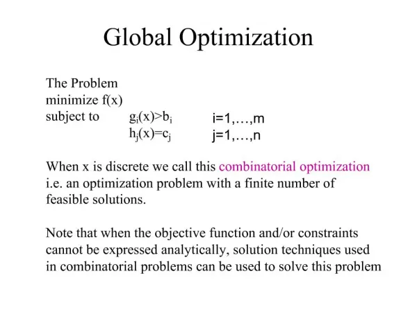
This document explores advanced data flow analysis techniques for compiler optimization, focusing on the examination of variable definitions and usage beyond basic blocks. It discusses optimizing transformations, including common subexpression elimination, loop-invariant code motion, constant folding, and more. It details the iterative algorithms over control flow graphs, highlighting the concepts of live variable analysis and reaching definitions. The analysis methods described facilitate improved code generation by allowing compilers to optimize using comprehensive variable information.


Advanced Data Flow Analysis for Compiler Optimization Techniques
E N D
Presentation Transcript
Global optimization Honors Compilers April 16th 2002
Data flow analysis • To generate better code, need to examine definitions and uses of variables beyond basic blocks. With use-definition information, various optimizing transformations can be performed: • Common subexpression elimination • Loop-invariant code motion • Constant folding • Reduction in strength • Dead code elimination • Basic tool: iterative algorithms over graphs
The flow graph • Nodes are basic blocks • Edges are transfers (conditional/unconditional jumps) • For every node B (basic block) we define the sets • Pred (B) and succ (B) which describe the graph • Within a basic block we can easily single pass) compute local information, typically a set • Variables that are assigned a value : def (B) • Variables that are operands: use (B) • Global information reaching B is computed from the information on all Pred (B) (forward propagation) or • Succ (B) (backwards propagation)
Example: live variable analysis • Definition: a variable is a live if its current value is used subsequently in the computation • Use: if a variable is not live on exit from a block, it does not need to be saved (stored in memory) • Livein (B) and Liveout (B) are the sets of variables live on entry/entry from block B. • Liveout (B) = livein (n) over all n ε succ (B) • A variable is live on exit from B if it is live in any successor of B • Livein (B) = liveout (B) use (B) – defs (B) • A variable is live on entrance if it is live on exit or used within B • Live (Bexit) = φ • On exit nothing is live
Liveness conditions x, y live z :=.. ..x * 3 y, z live ..z -2 ..y+1
Example: reaching definitions • Definition: the set of computations (quadruples) that may be used at a point • Use: compute use-definition relations. • In (B) = out (p) for all p ε pred (B) • A computation is reaches the entrance to a block if it reached the exit of a predecessor • Out (B) = in (B) + gen (B) – kill (B) • A computation reaches the exit if it is reaches the entrance and is not recomputed in the block, or if it is computed locally • In (Bentry) = φ • Nothing reaches the entry to the program
Iterative solution • Note that the equations are monotonic: if out (B) increases, in (B’) increases for some successor. • General approach: start from lower bound, iterate until nothing changes. Initially in (b) = φ for all b, out (b) = gen (b) change := true; while change loop change := false; forall b ε blocks loop in (b) = out (p), forall p ε pred (b); oldout := out (b); out (b) := gen (b) in (b) – kill (b); if oldout /= out (b) then change := true; end if; end loop; end loop;
Workpile algorithm • Instead of recomputing all blocks, keep a queue of nodes that may have changed. Iterate until queue is empty: while not empty (queue) loop dequeue (b); recompute (b); if b has changed, enqueue all its successors; end loop; • Better algorithms use node orderings.
Example: available expressions • Definition: computation (triple, e.g. x+y) that may be available at a point because previously computed • Use: common subexpression elimination • Local information: • exp_gen (b) is set of expressions computed in b • exp_kill (b) is the set of expressions whose operands are evaluated in b • in (b) = ∩ out(p) for all p ε pred (b) • Computation is available on entry if it is available on exit from all predecessors • out (b) = exp_gen (b) in (b) – exp_kill (b)
Iterative solution • Equations are monotonic: if out (b) decreases, in (b’) can only decrease, for all successors of b. • Initially • in (bentry) = φ, out (bentry) = e_gen (bentry) • For other blocks, let U be the set of all expresions, then • out (b) = U- e_kill (b) • Iterate until no changes: in (b) can only decrease. Final value is at most the empty set, so convergence is guaranteed in a fixed number of steps.
Use-definition chaining • The closure of available expressions: map each occurrence (operand in a quadruple) to the quadruple that may have generated the value. • ud (o): set of quadruples that may have computed the value of o • Inverse map: du (q) : set of occurrences that may use the value computed at q.
finding loops in flow-graph • A node n1 dominates n2 if all execution paths that reach n2 go through n1 first. • The entry point of the program dominates all nodes in the program • The entry to a loop dominates all nodes in the loop • A loop is identified by the presence of a (back) edge from a node n to a dominator of n • Data-flow equation: • dom (b) = ∩ dom (p) forall p ε b • a dominator of a node dominates all its predecessors
Loop optimization • A computation (x op y) is invariant within a loop if • x and y are constant • ud (x) and ud (y) are all outside the loop • There is one computation of x and y within the loop, and that computation is invariant • A quadruple Q that is loop invariant can be moved to the pre-header of the loop iff: • Q dominates all exits from the loop • Q is the only assignment to the target variable in the loop • There is no use of the target variable that has another definition. • An exception may now be raised before the loop
Strength reduction • Specialized loop optimization: formal differentiation • An induction variable in a loop takes values that form an arithmetic series: k = j * c0 + c1 • Where j is the loop variable j = 0, 1, … , c and k are constants. J is a basic induction variable. • Can compute k := k + c0, replacing multiplication with addition • If j increments by d, k increments by d * c0 • Generalization to polynomials in j: all multiplications can be removed. • Important for loops over multidimensional arrays
Induction variables • For every induction variable, establish a triple (var, incr, init) • The loop variable v is (v, 1, v0) • Any variable that has a single assignment of the form k := j* c0 + c1 is an induction variable with (j, c0 * incrj, c1+ c0 * j0 ) • Note that c0 * incrj is a static constant. • Insert in loop pre-header: k := c0 * j0 + c1 • Insert after incrementing j: k := k + c0 * incrj • Remove original assignment to k
Global constant propagation • Domain is set of values, not bit-vector. • Status of a variable is (c, non-const, unknown) • Like common subexpression elimination, but instead of intersection, define a merge operation: • Merge (c, unknown) = c • Merge (non-const, anything) = non-const • Merge (c1, c2) = if c1 = c2 then c1 else non-const In (b) = Merge { out (p) } forall p ε pred (b) • Initially all variables are unknown, except for explicit constant assignments