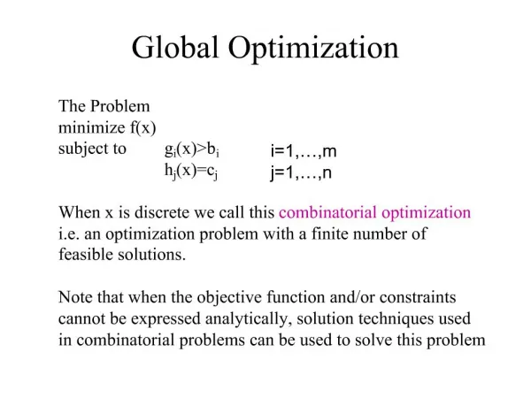
Global Optimization Techniques in Program Analysis
Learn about global flow analysis, constant propagation, and liveness analysis in program optimization as taught by Prof. Hilfinger in CS164. Dive into the intricacies of constant replacement conditions, undecidability of program properties, and conservative program analyses. Understand the importance of global dataflow analysis in solving optimization problems and how to apply global constant propagation effectively. Discover the fundamental principles behind global analysis methods and enhancing code efficiency through these advanced techniques.

Global Optimization Techniques in Program Analysis
E N D
Presentation Transcript
Global Optimization Lecture 27 (From notes by R. Bodik & G. Necula) Prof. Hilfinger CS164 Lecture 27
Administrative • HW #6 was posted online this evening. • Version #2 of project 3 files: representation now complete, but still a bit of work for me to do. Prof. Hilfinger CS164 Lecture 27
Lecture Outline • Global flow analysis • Global constant propagation • Liveness analysis Prof. Hilfinger CS164 Lecture 27
X := 3 Y := Z * W Q := 3 + Y Y := Z * W Q := 3 + Y Local Optimization Simple basic-block optimizations… • Constant propagation • Dead code elimination X := 3 Y := Z * W Q := X + Y Prof. Hilfinger CS164 Lecture 27
Global Optimization … extend to entire control-flow graphs X := 3 B > 0 Y := Z + W Y := 0 A := 2 * X Prof. Hilfinger CS164 Lecture 27
Global Optimization … extend to entire control-flow graphs X := 3 B > 0 Y := Z + W Y := 0 A := 2 * X Prof. Hilfinger CS164 Lecture 27
Global Optimization … extend to entire control-flow graphs X := 3 B > 0 Y := Z + W Y := 0 A := 2 * 3 Prof. Hilfinger CS164 Lecture 27
X := 3 B > 0 Y := Z + W X := 4 Y := 0 A := 2 * X Correctness • How do we know it is OK to globally propagate constants? • There are situations where it is incorrect: Prof. Hilfinger CS164 Lecture 27
Correctness (Cont.) To replace a use of x by a constant k we must know that: Constant Replacement Condition (CR): On every path to the use of x, the last assignment to x is x := k Prof. Hilfinger CS164 Lecture 27
Example 1 Revisited X := 3 B > 0 Y := Z + W Y := 0 A := 2 * X so replacing X by 3 is OK Prof. Hilfinger CS164 Lecture 27
X := 3 B > 0 Y := Z + W X := 4 Y := 0 A := 2 * X Example 2 Revisited so replacing X by 3 is not OK Prof. Hilfinger CS164 Lecture 27
Discussion • The correctness condition is not trivial to check • “All paths” includes paths around loops and through branches of conditionals • Checking the condition requires global analysis • An analysis of the entire control-flow graph for one method body Prof. Hilfinger CS164 Lecture 27
Global Analysis Global optimization tasks share several traits: • The optimization depends on knowing a property P at a particular point in program execution • Proving P at any point requires knowledge of the entire method body • Property P is typically undecidable ! Prof. Hilfinger CS164 Lecture 27
Undecidability of Program Properties • Rice’s theorem: Most interesting dynamic properties of a program are undecidable: • Does the program halt on all (some) inputs? • This is called the halting problem • Is the result of a function F always positive? • Assume we can answer this question precisely • Take function H and find out if it halts by testing function F(x) { H(x); return 1; } whether it has positive result • Syntactic properties are decidable ! • E.g., How many occurrences of “x” are there? • Theorem does not apply in absence of loops Prof. Hilfinger CS164 Lecture 27
Conservative Program Analyses • So, we cannot tell for sure that “x” is always 3 • Then, how can we apply constant propagation? • It is OK to be conservative. If the optimization requires P to be true, then want to know either • P is definitely true • Don’t know if P is true or false • It is always correct to say “don’t know” • We try to say don’t know as rarely as possible • All program analyses are conservative Prof. Hilfinger CS164 Lecture 27
Global Analysis (Cont.) • Global dataflow analysis is a standard technique for solving problems with these characteristics • Global constant propagation is one example of an optimization that requires global dataflow analysis Prof. Hilfinger CS164 Lecture 27
Global Constant Propagation • Global constant propagation can be performed at any point where CR condition holds • Consider the case of computing CR condition for a single variable X at all program points Prof. Hilfinger CS164 Lecture 27
Global Constant Propagation (Cont.) • To make the problem precise, we associate one of the following values with X at every program point Prof. Hilfinger CS164 Lecture 27
X = * X = 3 X = 3 X = 3 X = * X = * X := 3 B > 0 X = 4 X = 3 X = 3 Y := Z + W X := 4 Y := 0 A := 2 * X Example Prof. Hilfinger CS164 Lecture 27
Using the Information • Given global constant information, it is easy to perform the optimization • Simply inspect the x = _ associated with a statement using x • If x is constant at that point replace that use of x by the constant • But how do we compute the properties x = _ Prof. Hilfinger CS164 Lecture 27
The Idea The analysis of a complicated program can be expressed as a combination of simple rules relating the change in information between adjacent statements Prof. Hilfinger CS164 Lecture 27
Explanation • The idea is to “push” or “transfer” information from one statement to the next • For each statement s, we compute information about the value of x immediately before and after s Cin(x,s) = value of x before s Cout(x,s) = value of x after s (we care about values #, *, k) Prof. Hilfinger CS164 Lecture 27
Transfer Functions • Define a transfer function that transfers information from one statement to another • In the following rules, let statement s have immediate predecessor statements p1,…,pn Prof. Hilfinger CS164 Lecture 27
X = * Rule 1 if Cout(x, pi) = * for some i, then Cin(x, s) = * p2 p3 p1 p4 X = * X = ? X = ? X = ? s Prof. Hilfinger CS164 Lecture 27
X = * Rule 2 If Cout(x, pi) = c and Cout(x, pj) = d and d c then Cin (x, s) = * X = d X = ? X = c X = ? s Prof. Hilfinger CS164 Lecture 27
X = c Rule 3 if Cout(x, pi) = c for at least one i and is c or # for all i, then Cin(x, s) = c X = c X = # X = c X = # s Prof. Hilfinger CS164 Lecture 27
Rule 4 if Cout(x, pi) =# for all i, then Cin(x, s) = # X = # X = # X = # X = # X = # s Prof. Hilfinger CS164 Lecture 27
The Other Half • Rules 1-4 relate the out of one statement to the in of the successor statement • they propagate information forward across CFG edges • Now we need rules relating the in of a statement to the out of the same statement • to propagate information across statements Prof. Hilfinger CS164 Lecture 27
X = # X = # Rule 5 Cout(x, s) =# if Cin(x, s) = # s Prof. Hilfinger CS164 Lecture 27
X = ? X = c Rule 6 Cout(x, x := c) =c if c is a constant x := c Prof. Hilfinger CS164 Lecture 27
X = ? X = * Rule 7 Cout(x, x := f(…)) =* x := f(…) Prof. Hilfinger CS164 Lecture 27
X = a X = a Rule 8 Cout(x, y := …) =Cin(x, y := …) if x y y := . . . Prof. Hilfinger CS164 Lecture 27
An Algorithm • For every entry s to the program, set Cin(x, s) = * • Set Cin(x, s) = Cout(x, s) = # everywhere else • Repeat until all points satisfy 1-8: Pick s not satisfying 1-8 and update using the appropriate rule Prof. Hilfinger CS164 Lecture 27
X = * X = 3 X = 3 X = 3 X = 3 The Value # • To understand why we need #, look at a loop X := 3 B > 0 Y := Z + W Y := 0 A := 2 * X A < B Prof. Hilfinger CS164 Lecture 27
The Value # (Cont.) • Consider the statement Y := 0 • To compute whether X is constant at this point, we need to know whether X is constant at the two predecessors • X := 3 • A := 2 * X • But info for A := 2 * X depends on its predecessors, including Y := 0! Prof. Hilfinger CS164 Lecture 27
The Value # (Cont.) • Because of cycles, all points must have values at all times • Intuitively, assigning some initial value allows the analysis to break cycles • The initial value # means “So far as we know, control never reaches this point” Prof. Hilfinger CS164 Lecture 27
X = * X = # X = # 3 3 3 3 3 3 3 X = # X = # Example X := 3 B > 0 X = # Y := Z + W Y := 0 X = # X = # A := 2 * X A < B We are done when all rules are satisfied ! Prof. Hilfinger CS164 Lecture 27
Another Example X := 3 B > 0 Y := Z + W Y := 0 A := 2 * X X := 4 A < B Prof. Hilfinger CS164 Lecture 27
X = * X = # X = # 4 3 3 3 * 3 3 4 * 3 X = # X = # X = # Another Example X := 3 B > 0 X = # Y := Z + W Y := 0 X = # X = # A := 2 * X X := 4 A < B Must continue until all rules are satisfied ! Prof. Hilfinger CS164 Lecture 27
Orderings • We can simplify the presentation of the analysis by ordering the values # < c < * • Drawing a picture with “smaller” values drawn lower, we get * … a lattice … -1 0 1 # Prof. Hilfinger CS164 Lecture 27
Orderings (Cont.) • * is the largest value, # is the least • All constants are in between and incomparable • Let lub be the least-upper bound in this ordering • Rules 1-4 can be written using lub: Cin(x, s) = lub { Cout(x, p) | p is a predecessor of s } Prof. Hilfinger CS164 Lecture 27
Termination • Simply saying “repeat until nothing changes” doesn’t guarantee that eventually nothing changes • The use of lub explains why the algorithm terminates • Values start as # and only increase • # can change to a constant, and a constant to * • Thus, C_(x, s) can change at most twice Prof. Hilfinger CS164 Lecture 27
Termination (Cont.) Thus the algorithm is linear in program size Number of steps = Number of C_(….) values computed * 2 = Number of program statements * 4 Prof. Hilfinger CS164 Lecture 27
Liveness Analysis Once constants have been globally propagated, we would like to eliminate dead code After constant propagation, X := 3 is dead (assuming this is the entire CFG) X := 3 B > 0 Y := Z + W Y := 0 A := 2 * X Prof. Hilfinger CS164 Lecture 27
Live and Dead • The first value of x is dead (never used) • The second value of x is live (may be used) X := 3 X := 4 Y := X Prof. Hilfinger CS164 Lecture 27
Liveness A variable x is live at statement s if • There exists a statement s’ that uses x • There is a path from s to s’ • That path has no intervening assignment to x Prof. Hilfinger CS164 Lecture 27
Global Dead Code Elimination • A statement x := … is dead code if x is dead after the assignment • Dead statements can be deleted from the program • But we need liveness information first . . . Prof. Hilfinger CS164 Lecture 27
Computing Liveness • We can express liveness as a function of information transferred between adjacent statements, just as in copy propagation • Liveness is simpler than constant propagation, since it is a boolean property (true or false) Prof. Hilfinger CS164 Lecture 27
X = true Liveness Rule 1 Lout(x, p) = Ú { Lin(x, s) | s a successor of p } p X = ? X = ? X = true X = ? Prof. Hilfinger CS164 Lecture 27
X = true X = ? Liveness Rule 2 Lin(x, s) =true if s refers to x on the rhs …:= x + … Prof. Hilfinger CS164 Lecture 27