Download

1 / 36
360 likes | 489 Views
Individual and Social Production Possibilities and Indifference Curves. International Economics Professor Dalton ECON 317 – Spring 2012. Individual to Social Production Possibilities. Y/time.

E N D
Individual and Social Production Possibilities and Indifference Curves International Economics Professor Dalton ECON 317 – Spring 2012
Individual to Social Production Possibilities Y/time Slope shows marginal rate of transformation between X and Y - MRTx,y (how much it costs in Y to produce an X) An individual’s production possibilities frontier shows the quantities of goods, X and Y, that can be produced within a given time period while efficiently using the resources at hand. 30 Slope is 30/15 = 2 The marginal cost of X = 2Y The marginal cost of Y = 1/2 X X/time 15
Three Individual PPFs Y Y Y 180 Joe Sam Bill 100 30 30 X 150 X X 120 Which individual is the best producer of X? Which individual is the best producer of Y? It depends upon what is meant by “best”!
A person is said to have an absolute advantage in producing a good if he can produce more of the good than can another. A person is said to have a comparative advantage in producing a good if he can produce the good at a lower cost than another. Comparative and Absolute Advantage
Three Individual PPFsAbsolute Advantage Y Y Y 180 Joe Sam Bill 100 30 30 X 150 X X 120 Absolute Advantage: Good X Sam (150) Bill (120) Joe (30) Absolute Advantage: Good Y Bill (180) Sam (100) Joe (30)
Three Individual PPFsComparative Advantage Y Y Y 180 Joe Sam Bill 100 30 30 X 150 X X 120 Comparative Advantage: Good X Sam: 2/3 Y Joe: 1 Y Bill: 3/2 Y Comparative Advantage: Good Y Bill: 2/3 X Joe: 1 X Sam: 3/2 X
Building the Social PPF Y Y Y 180 Comparative Advantage: Good X Sam: 2/3 Y Joe: 1 Y Bill: 3/2 Y Bill Joe 310 30 30 X X 120 Y Sam 100 150 X X 300
Building the Social PPF • The Social PPF is the “summation” of all the individual agents’ PPFs in the economy, constructed by applying the principle of comparative advantage.
Many Person Social PPF Slope is flat at A. Low opportunity cost of X. Y/time A Slope is steep at B. High opportunity cost of X. B X/time
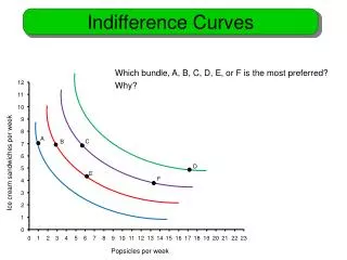
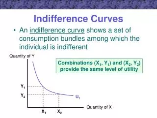
Characteristics 1. Fixed preferences 2. Negatively-sloped 3. Convex 4. Non-intersecting 5. Slope = Marginal Rate of Substitution (MRSxy) 6. Higher indifference curve represents greater utility Indifference Curves Y/time U3 U2 U1 X/time
The Marginal Rate of Substitution represents a trade-off ratio; the marginal benefit from a unit of one good in terms of another. Indifference Curves Y/time A 11 If the individual is at point A, an additional unit of X is worth 2Y. 9 B 3.2 U2 If the individual is at B, an additional X is worth 0.2 Y. 3 3 4 11 12 X/time
Budget Constraint • A budget constraint is negatively-sloped, reflecting the notion of opportunity cost - one must give up one good to get more of another. • The slope of a budget constraint measures the opportunity cost of one additional unit of a good in terms of the foregone units of the other good.
Budget Constraint • In consumer choice, the budget constraint usually consists of an income constraint reflecting relative prices of the two goods. • The budget constraint can also consist of the individual’s PPF, reflecting the individual’s MRT. • In either case, the slope of a budget constraint measures the opportunity cost of one additional unit of a good in terms of the foregone units of the other good.
C I Py A I 0 Px Budget Constraint What is the slope of the budget constraint? Slope equals rise over run. For an income constraint, slope equals I/Py divided by I/Px. (where I is income and Pj is the price of good j) I/Py/I/Px = Px/Py Y/time The slope of the budget constraint equals the price ratio Px/Py X/time
C Y A 0 X Budget Constraint What is the slope of the individual production possibility frontier? Slope equals rise over run. For an PPF, slope equals Y divided by X, and is the Marginal Rate of Transformation, MRTx,y. Y/time The slope of the budget constraint equals MRTx,y X/time
Here, MRSx,y > Px/Py (or MRTx,y). The individual can buy an additional X for less than the additional unit is valued. Choice: Combining Indifference Curves with Production Possibilities Y/time MC MB Here, MRSx,y < Px/Py (or MRTx,y). The individual would have to pay more than the additional unit of X is valued. U3 U2 U1 1 2 X/time
When the MRSx,y > Px/Py (or MRSx,y > MRTx,y) , the individual can make himself better off by selling a unit of Y to purchase additional units of X, since a unit of X is valued more highly than a unit of Y at the going prices. So long as this remains true, the individual continues to move “down” his budget constraint. Choice Y/time 1Y U3 U2 U1 1 3 X/time
When MRSx,y = Px/Py (or MRSx,y = MRTx,y), the individual will have reached a point where he can make himself no better off by a rearrangement of resources in X and Y consumption. Choice Y/time Y* U3 U2 U1 He will have maximized his utility! X* X/time
Starting from an original budget constraint … Changes inthe Budget Constraint Y/time Suppose that the price of X falls… The consumer can now buy more X if all income is spent on X… But can buy no more Y if all income is spent on Y… X/time The budget constraint rotates outward “around” the original Y-intercept
Starting from an original budget constraint … Changes inthe Budget Constraint Y/time Suppose that the price of X increases… The consumer can now buy less X if all income is spent on X… But can buy no more Y if all income is spent on Y… X/time The budget constraint rotates inward “around” the original Y-intercept
Starting from an original budget constraint … Changes inthe Budget Constraint Y/time Suppose that the price of Y falls… The consumer can now buy more Y if all income is spent on Y… But can buy no more X if all income is spent on X… X/time The budget constraint rotates outward “around” the original X-intercept
Starting from an original budget constraint … Changes inthe Budget Constraint Y/time Suppose that the price of Y increases… The consumer can now buy less Y if all income is spent on Y… But can buy no more X if all income is spent on X… X/time The budget constraint rotates inward “around” the original X-intercept
Starting from an original budget constraint … Changes inthe Budget Constraint Y/time Suppose that money income I increases… The consumer can now buy more Y if all income is spent on Y… and can buy more X if all income is spent on X… X/time The budget constraint shifts outward. Does the slope change? NO.
Starting from an original budget constraint … Changes inthe Budget Constraint Y/time Suppose that money income I decreases… The consumer can now buy less Y if all income is spent on Y… and can buy less X if all income is spent on X… X/time The budget constraint shifts inward. Does the slope change? NO.
Start from an original set of Indifference Curves (only one of which is shown). Changes inIndifference Curves Y/time If the individual is at point A, an additional unit of X is worth 2Y. A 11 9 Suppose that the individual’s preferences change so that X is now valued more highly (he prefers X relatively more)… 6 U2 Now the individual will value an additional unit of X at more than 2Y, say 5Y… 3 4 X/time The set of indifference curves will become steeper…
Start from an original set of Indifference Curves (only one of which is shown). Changes inIndifference Curves Y/time If the individual is at point A, an additional unit of X is worth 2Y. A 11 10 Suppose that the individual’s preferences change so that Y is now valued more highly (he prefers X relatively less)… U2 Now the individual will value an additional unit of X at less than 2Y, say 1Y… 3 4 11 12 X/time The set of indifference curves will become flatter…
Beginning from equilibrium, Changes in Behavior: Price Y/time suppose that Px falls. The budget constraint rotates outward around the Y-intercept… Y** Y* U3 U2 The consumer chooses a new X, Y combination: X**, Y** U1 X* X** X/time
Beginning from equilibrium, Changes in Behavior: Price Y/time suppose that Px rises. The budget constraint rotates outward around the Y-intercept… Y’ Y* U3 U2 The consumer chooses a new X, Y combination: X’, Y’ U1 X* X’ X/time
Beginning from equilibrium, suppose that Income rises. Changes in Behavior: Income Y/time The budget constraint shifts outward and the slope doesn’t change (why?) Y** Y* U3 U2 U1 The consumer chooses a new X, Y combination: X**, Y** X* X** X/time
As this graph what kind of goods are X and Y? Changes in Behavior: Income Y/time Both are normal goods. Y** Y* U3 U2 U1 X* X** X/time
Suppose, that instead, money income had fallen. Again that means a new equilibrium, and a new equilibrium combination of X’ and Y’. Changes in Behavior: Income Y/time Y* U3 Y’ U2 U1 X’ X* X/time
Start from an original equilibrium, A. Changes in Behavior: Preferences Y/time Suppose preferences become more favorable to X…the IC steepen. A Y* B Y** The individual now moves to a bundle favoring more X and Less Y, at B. X* X** X/time
Social Indifference Curves? • Can we sum up the preferences of individuals into a social indifference curve? • We could if we could measure the intensity of preferences independent of income levels, or measure utility directly. • But we can’t. • Further, Arrow’s Impossibility Theorem shows that there exists no rule that allows us to combine preferences without giving some one person in society totalitarian power over the resulting choice.
TANSTAASIC There ain’t no such thing as a Social Indifference Curve…(sometimes called a Social Welfare Function). But BE WARE, textbooks and journal articles often present graphs that pretend that we can aggregate individual preferences into a Social Preference Ordering – a Social Indifference Curve.
TANSTAASIC For a two good world, we can employ the fiction that the indifference curve represents the preferences of the marginal or representative individual in society. When we move to more than two goods, however, this fiction becomes untenable.
TANSTAASIC • Why use graphs that show Country PPFs and Country ICs? (that violate TANSTAASIC!) • As a short-hand for the more complicated process of actual price formation…that’s all. • Don’t commit the fallacy of misplaced concreteness.