Download
1 / 20
210 likes | 899 Views
Labor Supply From Indifference Curves. Overview.

E N D
Overview In this chapter we want to explore the economic model of labor supply. The model assumes that individuals try to maximize their happiness or utility. The basic choice people have in this context is find the level of income and leisure that gives them maximum utility. We will assume that time is either spent in leisure or labor. Thus, as the amount of leisure changes, the labor supply of the individual changes in the opposite direction.
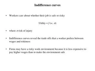
Utility maximization • The individual labor supply decision is analyzed in a framework of individual utility maximization. • In this framework the individual acquires utility by obtaining income from work, or doing things like hiking or going to the movies. • By working we can acquire goods and services and thus we obtain utility. • In the labor supply decision we will focus on two concepts: income and leisure.
Utility maximization • Income refers to the dollar amount we get from working. • The more income or leisure we have the more happy we are. In other words, both income and leisure add to our utility.
Tools • We are going to develop some tools called the budget constraint and indifference curves. • This tools are used by economists to understand labor supply decisions of individuals. • Indifference curves give a summary view of the individual’s subjective view of the goods we will talk about later: income and leisure. • The budget constraint gives a summary view of the amounts of income and leisure attainable by the individual in the market.
Diagram used in analysis income Income is measured on the vertical axis. Higher positions mean more income. Leisure A B Leisure is measured on the horizontal axis. As we move from A to B we are counting more hours of leisure(and less labor). Moving from B to A means we have more labor supplied.
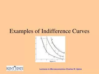
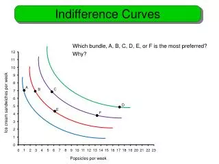
Indifference curves Indifference curves are constructed as an attempt to get a feel for how much utility people receive from various combinations of the income and leisure they obtain. Plus the curves help us compare how an individual would rate different combinations. A person will either prefer combination A to B, prefer B to A, or be indifferent between the two (like the two equally well). Here we will focus on indifference curves relating to peoples views on income and leisure.
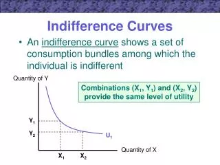
Indifference curves - definition • An indifference curve shows various combinations of income and leisure which will yield some specific level of utility or satisfaction for the individual. income This is a typical looking indifference curve. The individual is equally happy at point A or B or any other point on this indifference curve. A B leisure
Indifference curves - feature 1 • We assume more goods are preferred to less and thus indifference curves slope downward to the right. income Say the individual is at the point in the middle of the graph. Keep this in mind as we explore the following screens. 2 1 3 4 leisure
Indifference curves - feature 1 • If the individual is at the point in the diagram, then all those points in area 1 and on the boundary are more preferred because those points have either more of both items or more of one and the same amount of the other item compared to the point chosen. • Points in area 3 and the boundary are less preferred to the point in the diagram because the point chosen has more of both items.
Indifference curves - feature 1 • An individual may think that points in areas 2 and 4 are preferable, less preferred or equally desirable to the point indicated. • Since areas 2 and 4 are the only ones that could have a point of indifference to the chosen, the indifference curves must have negative slope.
Indifference curves - feature 2 • Indifference curves are said to be convex. • Part of the reason for this is that it is assumed that the amount of income one is willing to give up to get more leisure depends on how much of each the individual starts out with. The higher the amount of income one has, the more income they would be willing to give up to get one more unit of leisure.
Indifference curves - feature 2 income You can tell that point A has more income than at B. As the individual moves to one more unit of leisure from either point A or B, some income must be given up. But more is given up if point A is the initial point. A B Leisure (this line is for the graph) The point is the more you have of something(like income at point A compared to point B), the more you are willing to give up to acquire an additional unit of something else.
Indifference curves - feature 2 • The marginal rate of substitution(MRS) is the amount of income given up to obtain one more unit of leisure, while maintaining the same level of utility. • We an think of the MRS as a fraction: • MRS=(change in income)/(change in leisure). • In this sense, the MRS is the slope of the curve at various points. Note the slope changes from point to point. In absolute value the fraction gets smaller the farther down the curve one moves. This is another way of saying the curve gets flatter.
Marginal rate of substitution income Note that as we move from point L to M we give up some income, but get back some leisure. The changes in income and leisure do NOT have to be of the same amount (in fact income is measured in dollars and L is measured in hours so they can NOT be equal). L M Leisure
MRS continued Now when we give up income we lose utility and when we get more leisure we get more utility. Note that as we move along an indifference curve the changes in utility are equal in absolute value because in total utility does not change when we move along an indifference curve. The MRS = the negative of the slope
Indifference curves - feature 3 income Indifference Map Every point in the graph has one, and only one, indifference curve running through it. Curves farther out from the origin have more utility. leisure
Indifference curves - feature 4 income Indifference curves for an individual do not cross. Say they did, like in this diagram. Then individual would be indifferent to A and B, indifferent to A and C, and thus by logic should be indifferent to B and C. C A B leisure But C has more of both goods compared to B and thus C is preferred to B. So the curves can not cross for an individual.
Indifference curves - feature 5 • Different people can have different general shapes of indifference curves. Some are relatively steep and some are relatively flat. • On the next slide I will put two peoples’ indifference curves and they will cross. Before we said one individual’s curves could not cross.
Indifference curves - feature 5 income Note how Mr. A has a steeper curve than Mr. B. From the point where the curves cross if both give up a unit of leisure, note how Mr. A has to give up Mr. A Mr. B leisure more income to make up for the loss of leisure than Mr. B. Mr. A has a stronger preference for leisure than Mr. B. The textbook calls Mr.B a workaholic and Mr. A a leisure lover. These are relative terms. Mr. B is relatively more of a workaholic.