Download
1 / 17
170 likes | 197 Views
Coestimating models of the large-scale internal, external, and corresponding induced Hermean magnetic fields. Michael Purucker and Terence Sabaka Raytheon @ Planetary Geodynamics Lab, GSFC. Outline. Comparative magnetic planetology Flybys: Placing bounds & Ideal body theory

E N D
Coestimating models of the large-scale internal, external, and corresponding induced Hermean magnetic fields Michael Purucker and Terence Sabaka Raytheon @ Planetary Geodynamics Lab, GSFC
Outline • Comparative magnetic planetology • Flybys: Placing bounds & Ideal body theory • Spectra & depth to magnetic source • Crustal magnetic fields? • Secular variation of core field? • Parameterization of terrestrial model • Proposed parameterization of Hermean model
One flyby does not a model make • Geophysical explorationists have long relied on simple rules that place bounds on the parameters of the source region. • Mathematical basis now systematized in the theory of ideal bodies (Parker, 1974, 1975, 2003)
Ideal body theory examples Mars (Parker, 2003) If magnetization of Mars is confined to a 50-km thick layer, it must be magnetized with an intensity of at least 4.76 A/m, irrespective of its direction. Moon (Nicholas, Purucker, and Sabaka, 2007) Used to constrain the origin of the Reiner Gamma lunar swirl. Mercury (Purucker) Using the maximum magnetic fields measured at the Mariner 10 encounters, if the magnetization is crustal and confined to a 50-km thick layer it must be magnetized with an intensity of at least 3.2 A/m, irrespective of its direction.
Spectra & Depth to magnetic source • Magnetic source depth (of core or crustal fields) can be estimated using a spectral approach, either with gridded or profile data. Voorhies, Sabaka and Purucker, 2002 Power Degree
Crustal magnetic fields Although the remanent magnetization required to explain the Mariner 10 results is less than that required to explain the Martian results, typical remanent magnetic fields have a coherence length that is small compared to the diameter of the planet. A spherical shell magnetized by an arbitrary internal field produces no field outside of the shell. Geologic processes that may leave a magnetic field signature include faulting and impact.
Processes with possible magnetic signatures Lobate compressional scarps Caloris impact
Secular variation of core field • A dynamo field should undergo secular variation, although perhaps not on a time scale amenable to our observation campaign. The character of the time variation provides clues as to the energy source driving the dynamo. • The detection of such changes is not expected to be easy in the presence of time-varying magneospheric fields. • A comprehensive (CM) approach is necessary to separate these multiple fields. • The terrestrial CM parameterizes the secular variation with B-splines, and has been successful at detecting the known sequence of geomagnetic jerks, and the expansion of the South Atlantic anomaly since the beginning of the Space age.
Parameterization of terrestrial CM model Goal: To better characterize the magnetic fields of interior origin by coestimating all the major magneitc fields in the quiet-time near-Earth environment.
Details of parameterization • Core & Lithosphere: Negative gradient of a potential function represented by a degree and order 65 internal spherical harmonic expansion in geographic coordinates, with SV represented by cubic B-spline through degree and order 13 with 2.5 year knot spacing. Observatory static vector bias solution. • Ionosphere: Currents assumed to flow in thin spherical shell at 110 km alt. Radial continuity. Quasi-dipole coordinate system (Richmond et al.). Induced component represented by an a-priori, four-layer, 1-D, radial-varying conductivity model derived from Sq and Dst data at selected European observatories (Olsen). Influence of solar activity controlled by an amplification factor (F10.7 used). • Magnetosphere: External spherical harmonic expansion in dipole coordinates, with regular daily and seasonal periodicities. Ring current variability modeled as a linear function of Dst.
Terrestrial example 1 Main sources of terrestrial field
Terrestrial example 2 Recovery of large scale Region 1 & 2 current system structure
Terrestrial Parameterization (User end) Planetary-mag.net Interactive web application
Proposed parameterization • Coestimation of large-scale internal, external, and corresponding induced fields • Large-scale and persistent toroidal magnetic fields that impinge the sampling shell of the satellite. • Basis functions: Spherical harmonics in appropriate coordinate systems, supplemented by cubic B-splines for time-variable fields • Necessary supplementary information • Anisotropic weighting of vector data • Use of priors
External field parameterization • Magnetopause currents • Tail Currents • FAC’s, if persistent • ???