An Introduction to Artificial Intelligence
620 likes | 740 Views
In this lecture, we explore how artificial intelligence agents can systematically determine actions based on potential outcomes. We discuss problem-solving agents, types of problems, and the formulation of goals and actions. Using examples like navigating from Arad to Bucharest in Romania and solving the vacuum world dilemma, we illustrate key concepts such as states, actions as transitions, and the importance of abstracting complex real-world scenarios. The session also covers basic search algorithms and strategies to define and evaluate problem-solving approaches in AI.

An Introduction to Artificial Intelligence
E N D
Presentation Transcript
An Introduction to Artificial Intelligence Lecture 3: Solving Problems by Sorting Ramin Halavati (halavati@ce.sharif.edu) • In which we look at how an agent can decide what to do by systematically considering the outcomes of various sequences of actions that it might take.
Outline • Problem-solving agents (Goal Based) • Problem types • Problem formulation • Example problems • Basic search algorithms
Assumptions • World States • Actions as transitions between states • Goal Formulation: A set of states • Problem Formulation: • The sequence of required actions to move from current state to a goal state
Example: Romania • On holiday in Romania; currently in Arad. • Flight leaves tomorrow from Bucharest • Formulate goal: • be in Bucharest • Formulate problem: • states: various cities • actions: drive between cities • Find solution: • sequence of cities, e.g., Arad, Sibiu, Fagaras, Bucharest
Setting the scene… • Problem solving by searching • Tree of possible actions sequences. • Knowledge is Power! • States • State transfers
Example: Vacuum World • Single-state Problem: • You know all. • Start in #5 • Solution?[Right, Clean]
Example: vacuum world • Multiple State Problem • Sensorless • Start in {1,2,3,4,5,6,7,8} • Solution? [Right, Clean, Left, Clean]
Example: vacuum world • Contingency • Nondeterminism: Cleaning may dirty a clean carpet. • Partially observable: Location, dirt at current location. • Percept: [L, Clean], i.e., start in #5 or #7Solution?[Right, if dirt then Clean]
Single-state problem formulation A problem is defined by four items: • initial state e.g., "at Arad" • actions or successor functionS(x) = set of action–state pairs • e.g., S(Arad) = {<Arad Zerind, Zerind>, <Arad Timisoara, Timisoara>, …} • goal test, can be • explicit, e.g., x = "at Bucharest" • implicit, e.g., Checkmate(x) • path cost (additive) • e.g., sum of distances, number of actions executed, etc. • c(x,a,y) is the step cost, assumed to be ≥ 0 • A solution is a sequence of actions leading from the initial state to a goal state
Selecting a state space • Real world is absurdly complex state space must be abstracted for problem solving • (Abstract) state = set of real states • (Abstract) action = complex combination of real actions • e.g., "Arad Zerind" represents a complex set of possible routes, detours, rest stops, etc. • For guaranteed realizability, any real state "in Arad“ must get to some real state "in Zerind" • (Abstract) solution = • set of real paths that are solutions in the real world • Each abstract action should be "easier" than the original problem
Vacuum world state space graph • States?Dirt and robot location • Actions?Left, Right, Clean • Goal test?No dirt at all locations • Path cost?1 per action
Example: The 8-puzzle • States?Locations of tiles • Actions?Move blank left, right, up, down • Goal test?Given • Path cost?1 per move
Example: robotic assembly • States? real-valued coordinates of robot joint angles parts of the object to be assembled • Actions? continuous motions of robot joints • Goal test? complete assembly • Path cost? time to execute
Example Cryptarithmatic FORTY Solution: 29786 F=2, + TEN + 850 O=9, + TEN + 850 R=7, ------- ----- etc. SIXTY 31486 • States? A cryptharithmetic puzzle w/ some letters replaced with digits. • Actions? Replacing a letter with an unused digit. • Goal test? Puzzle contains only digits. • Path cost? ZERO. All solutions equally valid.
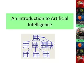
Tree search algorithms • Basic idea: • offline, simulated exploration of state space by generating successors of already-explored states (a.k.a.~expanding states)
Implementation: states vs. nodes • A state is a (representation of) a physical configuration • A node is a data structure constituting part of a search tree includes state, parent node, action, path costg(x), depth • The Expand function creates new nodes, filling in the various fields, using the SuccessorFnof the problem to create the corresponding states.
Search strategies • A search strategy is defined by picking the order of node expansion • Strategies are evaluated along the following dimensions: • completeness: does it always find a solution if one exists? • time complexity: number of nodes generated • space complexity: maximum number of nodes in memory • optimality: does it always find a least-cost solution? • Time and space complexity are measured in terms of • b: maximum branching factor of the search tree • d: depth of the least-cost solution • m: maximum depth of the state space (may be ∞)
Uninformed search strategies • Uninformed search strategies use only the information available in the problem definition • Breadth-first search • Uniform-cost search • Depth-first search • Depth-limited search • Iterative deepening search
Breadth-first search • Expand shallowest unexpanded node • Implementation: • fringe is a FIFO queue, i.e., new successors go at end
Breadth-first search • Expand shallowest unexpanded node • Implementation: • fringe is a FIFO queue, i.e., new successors go at end
Breadth-first search • Expand shallowest unexpanded node • Implementation: • fringe is a FIFO queue, i.e., new successors go at end
Breadth-first search • Expand shallowest unexpanded node • Implementation: • fringe is a FIFO queue, i.e., new successors go at end
Properties of breadth-first search • Complete?Yes (if b is finite) • Time?1+b+b2+b3+… +bd + b(bd-1) = O(bd+1) • Space?O(bd+1) (keeps every node in memory) • Optimal? Yes (if cost = 1 per step)
Uniform-cost search • Expand least-cost unexpanded node • Implementation: • fringe = queue ordered by path cost • Equivalent to breadth-first if step costs all equal
Uniform-cost search Sample 75 X 140 118
Uniform-cost search Sample 146 X X 140 118
Uniform-cost search Sample 146 X X 140 X 229
Uniform-cost search • Complete? Yes • Time? # of nodes with g ≤ cost of optimal solution, O(bceiling(C*/ ε)) where C* is the cost of the optimal solution • Space? # of nodes with g ≤ cost of optimal solution, O(bceiling(C*/ ε)) • Optimal? Yes
Depth-first search • Expand deepest unexpanded node • Implementation: • fringe = LIFO queue, i.e., put successors at front
Depth-first search • Expand deepest unexpanded node • Implementation: • fringe = LIFO queue, i.e., put successors at front
Depth-first search • Expand deepest unexpanded node • Implementation: • fringe = LIFO queue, i.e., put successors at front
Depth-first search • Expand deepest unexpanded node • Implementation: • fringe = LIFO queue, i.e., put successors at front
Depth-first search • Expand deepest unexpanded node • Implementation: • fringe = LIFO queue, i.e., put successors at front
Depth-first search • Expand deepest unexpanded node • Implementation: • fringe = LIFO queue, i.e., put successors at front
Depth-first search • Expand deepest unexpanded node • Implementation: • fringe = LIFO queue, i.e., put successors at front
Depth-first search • Expand deepest unexpanded node • Implementation: • fringe = LIFO queue, i.e., put successors at front
Depth-first search • Expand deepest unexpanded node • Implementation: • fringe = LIFO queue, i.e., put successors at front
Depth-first search • Expand deepest unexpanded node • Implementation: • fringe = LIFO queue, i.e., put successors at front
Depth-first search • Expand deepest unexpanded node • Implementation: • fringe = LIFO queue, i.e., put successors at front
Depth-first search • Expand deepest unexpanded node • Implementation: • fringe = LIFO queue, i.e., put successors at front
Properties of depth-first search • Complete? No: fails in infinite-depth spaces, spaces with loops • Modify to avoid repeated states along path complete in finite spaces • Time?O(bm): terrible if m is much larger than d • but if solutions are dense, may be much faster than breadth-first • Space?O(bm), i.e., linear space! • Optimal? No
Depth-limited search = depth-first search with depth limit l, i.e., nodes at depth l have no successors • Recursive implementation: