Download

1 / 51
510 likes | 535 Views
This study explores stereo-dynamic effects in NO-rare gas collisions using quasi-quantum treatment and ion imaging experiments. The differential cross sections and parity effects are analyzed to provide insights into the steric asymmetry. By developing a quasi-quantum mechanical model, the researchers aim to better understand the physical mechanisms governing these interactions.

E N D
Quantum Interference as the Source of Stereo-Dynamic Effects in NO-Rare Gas Scattering A. Gijsbertsen, C.A. Taatjes*, D.W. Chandler*, H.V. Linnartz and S. Stolte Department of Physical Chemistry, De Boelelaan 1083, 1081 HV Amsterdam vrije Universiteit amsterdam *Combustion Research Facility, Sandia National Laboratories, Livermore, California 94550
Outline • Introduction • Quasi-Quantum Treatment • Ion Imaging Experiments • Differential Cross Sections (DCSs) • Parity Effects • Conclusions and Outlook
Introduction oriented 21/2 NO ( j = ½, = -1) + R 21/2 NO ( j’, ’ ) + R With R = Ar, He, D2,...
Introduction The NO molecules are rotationally excited due to collisions with rare gas atoms. Laser Induced Fluorescence (LIF) is used to measure the amount of molecules present in a particular rotational state after collision: it provides the total collision cross section . The steric asymmetry S is given by:
NO-Ar, Etr 500 cm-1 Sif NO-He, Etr 500 cm-1 Sif Introduction N-end j = odd dominates O-end j = even dominates
Introduction A close coupling treatment reproduces experimental Sif: - it showed that the oscillatory Sif is due to the anisotropy in the hard shell of R-NO potential*. - it offers no explanation for undulative dependence upon j’ ! Our goal is to construct a quasi-quantum mechanical model to: obtain more information about the physical background of the steric asymmetry *(Alexander, Stolte, J. Chem. Phys. 112 (2000) 437)
Introduction Rainbow undulation for atom-atom scattering are caused by the pathway interference of 3 “rays” with different impact parameters: H. Pauly et al. 1966
Quasi-Quantum treatment The state selected wave function contains all NO orientations. Assuming a hard shell the scattering angle is determined only by the angle between the surface normal and the incoming momentum ħk. At fixed an infinite number of “rays” with different impact parameters b interfere, due to different path lengths.
Quasi-Quantum treatment Equipotential shell surface at Etr.
Quasi-Quantum treatment ^ ^ The kinematic apse n points perpendicularly to the hard shell. The projection of the rotational angular momentum (mj) is conserved along n. The difference between the “hard shell” trajectory and the virtual pathway through the center of mass yields the phase shift . ^
k’ (j = 0) k’ (j = 1) k’ (j = 2) k’ k’ (j = 3) k’ (j = 4) k’|| (= k||) k k k|| Quasi-Quantum treatment Assuming a hard shell, only the momentum component perpendicular to the shell (k) can be transformed into rotation. The scattering angle depends on:1. Spacing between rotational states 2. Angle between incoming momentum and apse.
Quasi-Quantum treatment The phase shift for several rotational states, as function of n. In this case cos()=-1. O-end N-end
Quasi-Quantum treatment The asymptotic solution of the Schrödinger equation at large distance, can be expressed as: The differential cross section relates to the dimensionless scattering amplitude: Remind, in the hard shell model, mj is conserved along the kinematic apse: mj’ =mj in the apse frame. Vdiff is ignored, so ’=.
Quasi Quantum treatment The scattering amplitude resulting from the hard shell model can be expressed as: with: Where w takes care of the non-isotropic shape of the shell: The conservation of flux is taken care of by introducing C() Note the elimination of the quantum numbers l and l’ !
Quasi Quantum treatment Flux conservation correction C()2
Quasi Quantum treatment Note that: After some algebra one finds: The distinguishes between the orientations. If positive Head collisions If negative Tail collisions
Quasi Quantum treatment The orientation dependent DCS can be written as: in which “+” denotes N-end and “–” O-end collision; Note that: From which follows: ! Increasing j’ j’+1, switches the orientation preference!
Quasi Quantum treatment O-end preference max cos(w) cos(w)
Quasi Quantum treatment A non-oriented NO wave function has parity : the DCS follows as: Note parity-pairs of similar DCSs, that can be observed: etc.
226 nm, 1 mJ 308 nm, 5 mJ He Hexapole NO source chamber NO collision chamber He source dye laser XeCl excimer laser Experiments Hexapole state selected NO collides with He at Ecoll 500 cm-1: Crossed 1+1’ REMPI detection excitation 226 nm ionization 308 nm NO (j=½, =½, =-1) NO ( j’, ’, ’ )
Experiments To test our setup, some 2% NO was seeded in the He beam. The NO beam consists of 16 % NO in Ar. This image reflects the velocity distributions for both our pulsed beams. vNO vHe
Experiments Parity conserving: p’ = p = - 1 j’ = 1.5 j’ = 2.5 j’ = 3.5 j’ = 4.5 j’ = 5.5 j’ = 6.5 * * j’ = 7.5 j’ = 8.5 j’ = 9.5 j’ = 10.5 j’ = 11.5 j’ = 12.5 Marked images are from Q-branch transitions that are more sensitive to rotational alignment and show more asymmetry. These images were omitted for the extraction of the DCS.
Experiments Parity breaking: p’ = - p = 1 j’ = 1.5 j’ = 2.5 j’ = 3.5 j’ = 4.5 j’ = 5.5 j’ = 6.5 * * * * * j’ = 7.5 j’ = 8.5 j’ = 9.5 j’ = 10.5 j’ = 11.5 j’ = 12.5
Parity conserving: p’ = p = - 1, DCSs [Å2] j’=1.5 [Å2] j’=2.5 [Å2] j’=3.5 [o] [o] [o] [Å2] j’=4.5 [Å2] j’=5.5 [Å2] j’=6.5 [o] [o] [o]
Parity conserving: p’ = p = - 1, DCSs [Å2] j’=7.5 [Å2] j’=8.5 [Å2] j’=9.5 [o] [o] [o] [Å2] [Å2] [Å2] j’=10.5 j’=11.5 j’=12.5 [o] [o] [o]
Parity breaking: p’ = - p = 1, DCSs [Å2] j’=1.5 [Å2] j’=2.5 [Å2] j’=3.5 [o] [o] [o] [Å2] j’=4.5 [Å2] j’=5.5 [Å2] j’=6.5 [o] [o] [o]
Parity breaking: p’ = - p = 1, DCSs j’=7.5 j’=8.5 j’=9.5 [Å2] [Å2] [Å2] [o] [o] [o] j’=10.5 j’=11.5 [Å2] j’=12.5 [Å2] [Å2] [o] [o] [o]
p’ = p = - 1 p’ = - p = 1 p’ = p = - 1 Parity Effects Recall that the Quasi Quantum Treatment yields the following propensity rule depending on the parity These parity-pairs of similar DCSs are seen in experimental results, the ratios within the pairs can be verified using HIBRIDON results.
Parity Effects The ratios between differential cross sections within parity pairs, is close to what the Quasi- Quantmum Treatment (QQT) predics. For large j the agreement becomes worse.
Conclusions and Outlook • Quasi quantum mechanical treatment that eliniminates l and l’ appears to be feasible for inelastic scattering. • The oscillatory dependence of S upon j’ can be explained as a quantum interference that invokes the repulsive part of the anisotropic potential. • An interference induced propensity rule of the DCS follows from our treatment and is seen experimentally. A physical interpretation of the DCSs emerges. • Measurements of orientation dependence of the DCSs will be attempted. • Is it possible to invert oriented DCSs to PESs?
Questions? j’ = 4.5, R21
velocity mapping Molecules in a certain rotational state (after collision) are ionized using 1+1’ REMPI and the ions are projected onto the detector, providing a 2D velocity distribution. + + + + repellor
velocity mapping The velocity distribution is recorded with a CCD camera. Ion images show the angular dependence of the inelastic collision cross sections of scattered NO (j’, ’, ’) molecules.
vNO vHe Some parameters Voltages: Vrepellor= 730 VVextractor = 500 V Sensitivity: S = 7.7 m/s/pixel NO beam velocity: vNO = 590 +/- 25 m/s He beam velocity: vHe= 1760 +/- 50 m/s Images are: - 80 x 80 pixels - averaged over 2000 laser shots (@ 10 Hz) Forward scattering ( = 0): Backward scattering ( = ):
DCS extraction • Extraction of differential cross sections (dcs’s) from • images: • Calculate the center(pixel) of the scattering circle • use intensity on an outer ring of the image as trial dcs • Use the trial dcs to simulate an image • Improve the dcs, minimizing the difference between simulated and measured image • Step 3 and 4 are repeated until the simulated an measured • images correspond well enough.
NO-He, P11 (’=1/2, ’=1) j’ = 1.5 j’ = 2.5 j’ = 3.5 j’ = 4.5 j’ = 5.5 j’ = 6.5 j’ = 7.5 j’ = 8.5 j’ = 9.5 j’ = 10.5 j’ = 11.5 j’ = 12.5 12-03-2004
NO-He R21 (’=1/2, ’=-1) j’ = 1.5 j’ = 2.5 j’ = 3.5 j’ = 4.5 j’ = 5.5 j’ = 6.5 j’ = 7.5 j’ = 8.5 j’ = 9.5 j’ = 10.5 j’ = 11.5 j’ = 12.5 12-03-2004
NO-He R11 Q21 (’=1/2, ’=1) j’ = 1.5 j’ = 2.5 j’ = 3.5 j’ = 4.5 j’ = 5.5 j’ = 6.5 j’ = 7.5 j’ = 8.5 j’ = 9.5 j’ = 10.5 j’ = 11.5 j’ = 12.5 15-03-2004
NO-He Q11 P21 (’=1/2, ’=-1) j’ = 1.5 j’ = 2..5 j’ = 3.5 j’ = 4.5 j’ = 5.5 j’ = 6.5 j’ = 7.5 j’ = 8.5 j’ = 9.5 j’ = 10.5 j’ = 11.5 j’ = 12.5 17-03-2004
NO-He P12 (’=3/2,’=1) j’ = 1.5 j’ = 2..5 j’ = 3.5 j’ = 4.5 j’ = 5.5 j’ = 6.5 j’ = 7.5 j’ = 8.5 j’ = 9.5 j’ = 10.5 j’ = 11.5 j’ = 12.5 15-03-2004
NO-He R22 (’=3/2,’=-1) j’ = 1.5 j’ = 2..5 j’ = 3.5 j’ = 4.5 j’ = 5.5 j’ = 6.5 j’ = 7.5 j’ = 8.5 j’ = 9.5 j’ = 10.5 j’ = 11.5 j’ = 12.5 15-03-2004
NO-He P22 Q12 (’=3/2,’=-1) j’ = 1.5 j’ = 2..5 j’ = 3.5 j’ = 4.5 j’ = 5.5 j’ = 6.5 j’ = 7.5 j’ = 8.5 j’ = 9.5 j’ = 10.5 j’ = 11.5 j’ = 12.5 15-03-2004
NO-He Q22 R12 (’=3/2,’=1) j’ = 1.5 j’ = 2..5 j’ = 3.5 j’ = 4.5 j’ = 5.5 j’ = 6.5 j’ = 7.5 j’ = 8.5 j’ = 9.5 j’ = 10.5 j’ = 11.5 j’ = 12.5 15-03-2004