TURBULENCE MODELING IN PHOENICS
430 likes | 809 Views
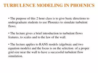
The purpose of this 2 hour class is to give basic directions to undergraduate students to use Phoenics to simulate turbulent flows. The lecture gives a brief introduction to turbulent flows features, to scales and to the law of the wall.

TURBULENCE MODELING IN PHOENICS
E N D
Presentation Transcript
The purpose of this 2 hour class is to give basic directions to undergraduate students to use Phoenics to simulate turbulent flows. • The lecture gives a brief introduction to turbulent flows features, to scales and to the law of the wall. • The lecture applies to RANS models (algebraic and two equation models) and the focus is on the selection of a proper grid size near the wall to have a successful turbulent flow simulation. TURBULENCE MODELING IN PHOENICS
Turbulent flow features • Fluctuatiation or Irregularity:turbulent flow is random ie not deterministic. The velocity fluctuates in all three directions, so does the pressure and temperature. • Turbulent flow is intrinsically transient. • Increased exchange of momentum: Diffusivity - spreading rate of jets, boundary layers etc. • Large Reynolds numbers; • Dissipation of kinetic energy to internal energy • Wide range of time and length scales • Almost all practical flows are turbulent.
Turbulent flow features: Eddies Side view of a turbulent boundary layer Water jet at symmetry plane, Re 2300 • Eddies are "packets" of fluid (identifiable flow structures) with different sizes ranging from macroscopic dimensions to the microscopic scale also known as Kolmogorov scale. • The large eddies are responsible to the transport of mass, momentum and heat. • The smallest eddies dissipate kinetic energy into heat through viscosity • The largest eddies scale to the characteristic flow dimension. • Boundary layer ~ boundary layer thickness; • pipe flow ~ pipe diamenter; • jet flow~ jet width and so forth.
Small eddies dissipates energy into heat (viscosity) Large eddies, contain kinetic energy Kolomogorov (1941) theory: the energy cascade • The energy is transferred from the mean flow to produce the large eddies. • The energy of the large eddies feed smaller eddies and these in turn transfer energy to smaller eddies yet. • This process results in a transfer of energy in the form of a cascade from larger eddies to smaller ones. • The smaller eddies dissipates the energy into heat due to the viscosity action. • The energy cascade suggest the multiple scales (size and frequencies) present in turbulent flow. This feature difficults the development of turbulence models. “Big-size whirls have little whirls that fed on their velocity Little whirls have lesser whirls and so on to viscosity”
Kolomogorov (1941) theory: length scales • Turbulence phenomenon has multiples scales: the largest contain energy and the smallest are responsible to dissipate energy. • The scales refers to the time, frequency spectrum or length sizes. • The ratio between the largest ‘l ‘ to the smallest scales ‘lk ‘is: • The length scale ratio impacts on the grid size definition necessary to encompass the largest to the smallest length scales. • Consider the turbulent flow in a plane channel: • For Re of 2.104 it is necessary a 40000 nodes grid to a channel volume equivalent to a one hydraulic diameter; for Re of 106 it is necessary a billion nodes grid!
Theeddies’ sizesand Re • The images below displays a jet flow with Re of 400 and 20000. Observe as Re increase the refinement of the length scale of the eddies due to Kolmogorov scale law: • The eddies’ smallest scale lk ratio for Re of 400 and 20000 is of 19:1
Prediction Methods l h = l/ReL3/4 Direct numerical simulation (DNS) Large eddy simulation (LES) Reynolds averaged Navier-Stokes equations (RANS) The focus of this presentation rests on RANS models only
Numerical Simulations : estimates of cost of fixed wing calculation Sample fixed wing of AR=10, Re=5E+06
Boussinesq hypothesis • Using the suffix notation where i, j, and k denote the x, y, and z directions respectively, viscous stresses are given by: • Many turbulence models are based upon the Boussinesq (1877) hypothesis: Reynolds stresses are linked to the mean rate of deformation. • Exceptions are DNS and partially LES.
Predicting the turbulent viscosity • The turbulent viscosity can be estimated by algebraic models or by solving a system of PDE. • Algebraic models (mixing length and LVEL) employs expressions similar to: T = C(dU/dy). They are computationally cheap but limited to very simple flows (pipe and boundary layers) • The 2nd category usually solves two equations to get T . So they are called by two equation models: k-, k-, k-l, k- RNG, etc. For k-: T = Ck2/ ; T derived by other 2 eq. models similarly follows k-. • There is also the Reynolds stress model which instead of estimate T it solves a system of six turbulent stress equations in order to get the Reynolds turbulent stress tensor. • The two equation models are largely applied to solve industrial problems. Very often the constants are tuned to specific cases to increase the accuracy.
Wall bounded flows • The presence of a wall damps the velocity and the turbulence near the wall region. • To capture the wall effect the turbulence models have to be modified near the wall. • The embodied wall models on the turbulence models are grid dependent. • The success of turbulent flow simulation starts on a careful choice of the grid spacing near the wall. • This presentation focus on near wall grid spacing selection to a successful simulation. To beginners this a potential area to make mistakes
Wall bounded flows and velocity damping near the wall • The presence of a wall damps the velocity and the turbulence near the wall region. • To capture the wall effect the turbulence models have to be modified near the wall. • The success of turbulent flow simulation starts on a careful choice of the grid spacing near the wall. Experimental turbulent boundary layer vel. Profiles for various pressure gradients. Coles 1968
Themeaning of thelayers • Inner layer: is the layer closest to the wall and is ruled by the fluid viscosity. The viscous length scale /u* is greater than the wall distance, or yu*/ = y+ << 1. On this region, u+ = y+ or = u/y. For modeling purposes the inner layer extends up to y+ = 5 • Overlap layer: is the region where the viscous action start loosing influence and the inertial effects increases. For modeling purposes this layer ranges from y+ = 5 up to 40. • Log layer: it is sufficiently far from the wall such that it is completely rulled by the inertial effects but close enough to the wall that the shear stress is uniform and equal to the wall shear stress! Usually the log layer ranges from y+ = 40 up to 200 • Outter layer: flow dominated by the eddies inertial effects, y+ > 200.
Inner + Buffer + Overlap Layers The velocity profiles near the wall are universally expressed in a dimensionless form: 200 5 40 Wall layers Outter Log Overlap Inner
Phoenicsturbulencemodels • Algebraic models: constant turbulent viscosity, mixing length, lvel. Lvel is the most popular, it can be applied starting from the inner layer or from the log layer. It is an algebraic expression which fits the near wall flow. These models are computationally cheap and delivers good results for channel or boundary layer flows. • Two equation models (standard) : refers to the k-e and variants. The distance from the wall of the first volume center has to lay within the log layer, 40 < y+ < 200. • Two equation models (low Re) : turbulent low Reynolds flows usually have the first node distance for 40 < y+ < 200 corresponding to a significant percentage of the domain (> 15%). To avoid numerical errors induced by the coarse grid it is preferred to starting integrating the flow starting from the wall. The first node must lay at y+ ~ 1 and at least 3 more volumes up to y+ < 5. This assures a smooth integration along the inner, overlap and log layer.
How to get good results from turbulence models • All models have limitations, one can not ask more than the model can deliver. • Algebraic models are the simplest and the most limited. Usually work well for pipe flows and boundary layers. • 2 equation models are more accurate than algebraic models but their constants do not have universally, it is possible for certain types of flow a better matching by tuning the constants. • 2 equation models considers flow in equilibrium: all the production of k is dissipated at the same point. Flow with sudden changes in direction are prone to be out of equilibrium. • In general, turbulent models demand a special care with the near wall mesh. If you get this wrong your simulation will fail.
WKSP #1-Turbulent flow develop. 2D channel • This WKSH deals with a turbulent flow development along a 2D channel flow. • The flow simulations will be done using Parabolic model (visit (1) and (2) links to further information). • Parabolic model apply only to one-way flows (no recirculation zones present). It will used along the WKSH because it is far more efficient than Elliptic model. • Along the WKSH will be supplied specific hints to set up a problem employing Parabolic model.
2D Channel dimensions & properties nwall (plate) y (b) no outlet specification Uniform GRID (c) NX=1 NY=28 NZ=80 Inlet H/2=0.05m Center line z (a) L = 10m (a) For parabolic model the main flow direction has to be aligned with the Z axis. (b) Parabolic flow has w component always along z > 0 direction, if happens to have w along z<0 it will fail. Due this feature it does not need specification of an outlet.
2D Channel dimensions & properties nwall (plate) y (b) no outlet specification Uniform GRID (c) NX=1 NY=24 NZ=80 Tolerance 10-6 Inlet H = 0.05m Center line z (a) L = 10m SETTING PARABOLIC MODEL: ACCESS THE VR-EDITOR BOXES AND SET: Model: choose parabolic (confined because is a channel) Ground: Parabolic model visits only one slab at a time and stores only the last slab. To provide full field storage go to VR-EDITOR box GRND and set IDSPA=1, IDSPB=1 and IDSPC=80 (always equal to NZ), IDSPD=1 Objects Inlet: Win = 10 m/s Re = 1.105 Inlet: 5% turbulence Plate: no slip, W=0 Output Pause atendofrun Storg.: YPLUS & STRS Model K-e • Properties • (~air) • = 1.0 kg/m3 • = 10-5 m2/s Numerics Iterac =1000 Relax (manual) 1; 1; 1; 0,5; 0,5 Phoenics variables
2D Channel Results – W velocity at z/D of 2D, 10D and 40D One may reproduce this figure using autoplot or get similar results employing ‘Ploting variable’ in VRVIEWER.
2D Channel Results – W center-line velocity overshoot experimental overshoot, see link 80D 64D 48D 16D 32D
2D Channel Results – Y+ & STRS • 1st volume distance correct: 40 < Y+ < 100. • 1st volume within Log Layer! • STRS = w/ • STRS fully developed = 0.192 • STRS Colebrook-White = 0.195 (1.5% off) 64D 48D 16D 32D
2D Channel Results – T, k and • Viscosity is a flow property: T = Ck2/ • Near the wall the ‘turbulent viscosity’ is 16 times greater than the molecular viscosity. • The largest changes on k and are near the wall. • At the centerline T is nearly 300 greater than . ENUT KE 80D 64D 48D 16D 32D EP
Phoenics adjustable constants for KE model • The choice of one constant value by other depends on previous knowledge about a specific flow and also knowledge about the meaning of the constants within the model, for KE visit turbulence.
Evaluating Cf thru Colebrook-White is possible to estimate, at the fully developed region: (i) 1st node distance from the wall (), (ii) number of volumes NY (uniformly distributed), (iii) STRS = w/. The last will be used to check the numerical solution. Keep in mind that H = 50mm. Exploring the grid sensitivity to Y+ and STRS KE – Low Re KE – Low Re KE - Standard KE - Standard
Workshop#1 – adjusting grids • Based on the table below select between ‘standard’ or ‘low Re’ KE models to cases where W = 1 and 50 m/s, also define a new NY. Do these changes on the previous Q1. • For reference, the previous case velocity is W = 10m/s or Re 105, • STRS Cole is the w/ value estimated by Colebrook-White for a fully developed flow. • Y+ = 1 thru 100 are the estimated first node distance to the wall.
Workshop – adjusting grids • Case W = 1m/s – ‘Low Re’ because the 1st volume for y+ = 40 would be at 7mm from the wall which is nearly 14% of the Y length. One can use a uniform grid or a more economical 2 region grid, the near wall grid extends up to y+ = 40 (~7mm) • Case W = 50m/s – Standard,
Workshop#2 – Flow in backward face step • A simple backward step flow challenges the 2 equation turbulence models because it has a shear layer, a recirculation zone, null wall shear stress point and a redeveloping boundary layer! • Compare the reattachment point position employing: k-e model, the Chen-Kim k-e model, the RNG k-e model, the k-omega model and the LVEL model.
Workshop#2 – Flow in backward face step • Load case T103 from library. Step height, H = 0.038m and ReH = 45000. Y L = 0.762 m or 20H Uin = 13 m/s 3H s = 0.1524 m or 4H H X • Change X grid regions to 10 and 60 cells (no power) • Change Y grid regions to 8 and 10 cells (the last with pwr 1.5 sym) • Start with the KE standard model • Store STRS and YPLUS
Workshop#2 – Flow in backward face step • Key flow features to explore are the wall shear stress and if possible the pressure distribution at the channel bottom wall. • The reattachment point is determined by the x distance where the wall shear is null. stress is null.
Workshop#2 – Flow in backward face step • Fill in the table
Workshop#2 – Flow in backward face step • Discuss the validity of the results in view (k-e model) of the y+ values Lower bound to two eq. Standard models • As the reattachment point is approached w 0 and Y+ 0 • Would you consider Low Re type models to capture the reattachment point? • If so use k-e low Re, same grid as before but modify Y 1st region to 60 cells, use pwr of + 1.6 and in Numerics set to 10000 sweeps
Workshop#2 – Flow in backward face step • The k-e low re apparently estimates nearly the same reattachment point position as predicted by k-e standard! • But the magnitude of the STRS has changed significantly! • In fact the k-e standard made wrong STRS estimations because it employed an inappropriate grid which resulted in y+ values lower than 40 at the neighborhood of reattachment point!
2D Channel dimensions & properties nwall (plate) y (b) no outlet specification Uniform GRID (c) NX=1 NY=28 NZ=80 Inlet H/2=0.05m Center line z (a) L = 10m (a) For parabolic model the main flow direction has to be aligned with the Z axis. (b) Parabolic flow has w component always along z > 0 direction, if happens to have w along z<0 it will fail. Due this feature it does not need specification of an outlet. (c) Parabolic model visits only one slab at a time and stores only the last slab. To provide full field storage go to VR-EDITOR box GRND and set IDSPA=1, IDSPB=1 and IDSPC=80 (always equal to NZ), IDSPD=1 ACCESS THE VR-EDITOR BOXES AND SET: Objects Inlet: Win = 10 m/s Re = 2.105 Inlet: 5% turbulence Plate: no slip, W=0 Output Pause atendofrun Storg.: YPLUS & STRS • Properties • (~air) • = 1.0 kg/m3 • = 10-5 m2/s Numerics Lsweep = 100 Relax (manual) Models K-E Phoenics variables