Download
1 / 38
380 likes | 557 Views
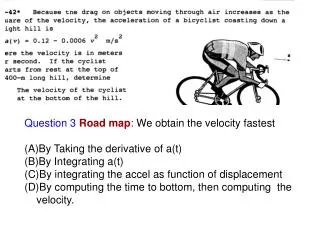
Question 3 Road map : We obtain the velocity fastest By Taking the derivative of a(t) By Integrating a(t) By integrating the accel as function of displacement By computing the time to bottom, then computing the velocity. Question 3 Road map : We obtain the velocity fastest

E N D
Question 3Road map: We obtain the velocity fastest • By Taking the derivative of a(t) • By Integrating a(t) • By integrating the accel as function of displacement • By computing the time to bottom, then computing the velocity.
Question 3Road map: We obtain the velocity fastest • By Taking the derivative of a(t) • By Integrating a(t) • By integrating the accel as function of displacement • By computing the time to bottom, then computing the velocity.
Chapter 12-5 Curvilinear Motion X-Y Coordinates
12.7 Normal and Tangential Coordinates ut : unit tangent to the path un : unit normal to the path
Normal and Tangential Coordinates Velocity Page 53
Normal and Tangential Coordinates ‘e’ denotes unit vector (‘u’ in Hibbeler)
‘e’ denotes unit vector (‘u’ in Hibbeler)
Polar coordinates ‘e’ denotes unit vector (‘u’ in Hibbeler)
Polar coordinates ‘e’ denotes unit vector (‘u’ in Hibbeler)
12.8 Polar coordinates In a polar coordinate system, the velocity vector can be written as v = vrur + vθuθ = rur + rquq. The term q is called A) transverse velocity. B) radial velocity. C) angular velocity. D) angular acceleration . . .
. . .
. . .
. . .
12.10 Relative (Constrained) Motion vA is given as shown. Find vB Approach: Use rel. Velocity: vB = vA +vB/A (transl. + rot.)
Vectors and Geometry r(t) y q q(t) x
Given: vectors A and B as shown. The RESULT vector is: • (A) RESULT = A - B • (B) RESULT = A + B • (C) None of the above
Given: vectors A and B as shown. The RESULT vector is: • (A) RESULT = A - B • (B) RESULT = A + B • (C) None of the above
12.10 Relative (Constrained) Motion V_truck = 60 V_car = 65 Make a sketch: A V_rel v_Truck B • The rel. velocity is: • V_Car/Truck = v_Car -vTruck
12.10 Relative (Constrained) Motion Make a sketch: A V_river v_boat B • The velocity is: • V_total = v+boat – v_river • V_total = v+boat + v_river
12.10 Relative (Constrained) Motion Make a sketch: A V_river v_boat B • The velocity is: • V_total = v+boat – v_river • V_total = v+boat + v_river
Example Vector equation: Sailboat tacking at 50 deg. against Northern Wind (blue vector) We solve Graphically (Vector Addition)
Example Vector equation: Sailboat tacking at 50 deg. against Northern Wind An observer on land (fixed Cartesian Reference) sees Vwind and vBoat . Land
12.10 Relative (Constrained) Motion Plane Vector Addition is two-dimensional. vA vB vB/A
Example cont’d: Sailboat tacking against Northern Wind 2. Vector equation (1 scalar eqn. each in i- and j-direction). Solve using the given data (Vector Lengths and orientations) and Trigonometry 500 150 i
Exam 1 • We will focus on Conceptual Solutions. Numbers are secondary. • Train the General Method • Topics: All covered sections of Chapter 12 • Practice: Train yourself to solve all Problems in Chapter 12
Exam 1 Preparation: Start now! Cramming won’t work. Questions: Discuss with your peers. Ask me. The exam will MEASURE your knowledge and give you objective feedback.
Exam 1 Preparation: Practice: Step 1: Describe Problem Mathematically Step2: Calculus and Algebraic Equation Solving