Dynamic Programming: Fibonacci Sequence & Matrix Multiplication
Learn how to compute Fibonacci sequence and optimal matrix-chain multiplication using dynamic programming. Understand key concepts like overlapping subproblems and optimal substructure. Discover efficient algorithms for solving complex optimization problems.

Dynamic Programming: Fibonacci Sequence & Matrix Multiplication
E N D
Presentation Transcript
Fibonacci Sequence • Compute
Fibonacci Sequence • Compute
Can we reuse the pre-computed results? • Yes, we can use memorandum to record the pre-computed results
Initialization 1 1 1 1 1 1 1 1 1 1 1 1 1 1 1 1
动态规划术语 重叠子结构、最优子结构 动态规划程序设计是对解最优化问题的一种途径、一种方法,而不是一种特殊算法。 在ACM里dp主要关心的是两个 1.状态 2.状态转移方程
1.选择状态:/*将问题发展到各个阶段时所处于的各种客观情况用不同的状态表示出来。当然,状态的选择要满足*/无后效性。1.选择状态:/*将问题发展到各个阶段时所处于的各种客观情况用不同的状态表示出来。当然,状态的选择要满足*/无后效性。 2.确定决策并写出状态转移方程:/*之所以把这两步放在一起,是因为决策和状态转移有着天然的联系,状态转移就是根据上一阶段的状态和决策来导出本阶段的状态。所以,如果我们确定了决策,状态转移方程也就写出来了。但事实上,我们常常是反过来做,根据相邻两段的各状态之间的关系来确定决策。*/ 3. 写出规划方程(包括边界条件):/*动态规划的基本方程是规划方程的通用形式化表达式。*/
Example 1 1 1 1 1 1 1 1 1 1 1 1 1 1 1 1
3 steps • 定义好状态 • 确定状态转移方程: • 确定边界条件:
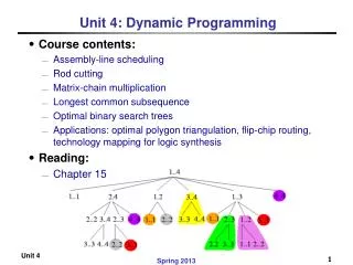
Matrix-chain multiplication • Goal. Given a sequence of matrices A1,A2,…,An, find an optimal order of multiplication. • Multiplying two matrices of dimensionp×q and q×r, takes time which is dominated by the number of scalar multiplication, which is pqr. • Generally. Ai has dimension pi-1×pi and we’d like to minimize the total number of scalar multiplications.
Example • Order 1 • Order 2
Brute force method • What if we check all possible ways of multiplying? How many ways of parenthesizing are there? • P(n): number of way of parenthesizing. Then P(1) =1 and for n≥2 • Fact • These numbers are called Catalan numbers. There are about 65 combinatorial interpretations in Stanley, Enumerative Combinatorics, Vol. 2
Optimal substructure • Notation. Ai..j represents Ai…Aj. • Any parenthesization of Ai..j where i < j must split into two products of the form Ai..k and Ak+1..j. • Optimal substructure. If the optimal parenthesization splits the product as Ai..k and Ak+1..j, then parenthesizations within Ai..k and Ak+1..j must each be optimal. • --We apply cut-and-paste argument to prove the optimal substructure property.
An optimal parenthesization’s structure • If the optimal parenthesization of A1 * A2 * … * An is split between Ak and Ak+1, then • The only uncertainty is the value of k • --Try all possible values of k. The one that returns the minimum is the right choice.
A recursive solution • Define m[i,j] as the minimum number of scalar multiplications needed to compute the matrix product Ai..j (We want the value of m[1,n].) • --If i = j, there is nothing to do, so that m[i,j] = 0; • --Otherwise, suppose that the optimal parenthesization split the product as Ai..kand Ak+1..j.
A recursive formulation • We would like to find the split that uses the minimum number of multiplications. Thus, • To obtain the actual parenthesization, keep track of the optimal k for each pair (i,j) as s[i,j].
Computing the Optimal Costs • --The recursive solution takes exponential time. (Easy proof by induction.) • Instead, use a dynamic program to fill in a table m[i,j]: • --Start by setting m[i,i]=0 for i = 1,…,n. • --Then compute m[1,2], m[2,3],…,m[n-1,n]. • --Then m[1,3], m[2,4],…,m[n-2,n],… • --… so on till we can compute m[1,n]. • The input a sequence p=<p0,p1,…,pn>, we use an auxiliary table s[1..n,1..n] that records which index of k achieved the optimal cost in computing m[i,j].
Example: DP for CMM • The optimal solution is ((A1(A2A3))((A4A5)A6)
Construct an Optimal Solution • The final matrix multiplication in computing A1..n optimally is A1..s[1,n]As[1,n]+1..n. s[1,s[1,n]] determines the last matrix multiplication in computing A1..s[1,n] and s[s[1,n]+1,n] determines the last matrix multiplication in computing As[1,n]+1..n.
Longest Common Subsequence • In biological applications, we often want to compare the DNA of two (or more) different organisms. • A strand of DNA consists of a string of molecules called bases, where the possible bases are adenine, guanine, cytosine, and thymine (A, G, C, T). • Comparison of two DNA strings • S1 = ACCGGTCGAGTGCGCGGAAGCCGGCCGAA • S2 = GTCGTTCGGAATGCCGTTGCTCTGTAAA • S3 = GTCGTCGGAAGCCGCCGAA • Comparison of two DNA strings • S1 = ACCGGTCGAGTGCGCGGAAGCCGGCCGAA • S2 = GTCGTTCGGAATGCCGTTGCTCTGTAAA
Longest Common Subsequence • Similarity can be defined in different ways: • -- Two DNA strands are similar if one is a substring of the other. • -- Two strands are similar if the number of changes needed to turn one into the other is small. • -- There is a third strand S3in which the bases in S3appear in each of S1and S2; these bases must appear in the same order, but not necessarily consecutively. The longer the strand S3 we can find, the more similar S1and S2 are. (we focus on this)
“a”not“the” Functional notation, but not a function Dynamic programming for LCS • Longest common subsequence (LCS) • -- Given two sequences x[1..m] and y[1..n], find a longest subsequence common to then both.
Brute-force LCS algorithm • Check every subsequence of x[1..m] to see if it is also a subsequence of y[1..n]. • Analysis • -- Checking = O(n) time per subsequence. • -- 2m subsequences of x (each bit-vector of length m determines a distinct subsequence of x). • -- Worst-case running time = O(n2m) • = exponential time
Towards a better algorithm • Simplification: • 1. Look at the length of a longest-common subsequence • 2. Extend the algorithm to find the LCS itself. • Notation: Denote the length of a sequence s by |s|. • Strategy: Consider prefixes of x and y. • -- Define c[i,j] = |LCS(x[1..i],y[1..j]| • -- Then, c[m,n] = |LCS(x,y)|
Simple Review • Elements of DP Algorithms • Optimal substructure • Overlapping Subproblem • Memoization • Longest Common Subsequence
“a”not“the” Functional notation, but not a function Dynamic programming for LCS • Longest common subsequence (LCS) • -- Given two sequences x[1..m] and y[1..n], find a longest subsequence common to then both.
Brute-force LCS algorithm • Check every subsequence of x[1..m] to see if it is also a subsequence of y[1..n]. • Analysis • -- Checking = O(n) time per subsequence. • -- 2m subsequences of x (each bit-vector of length m determines a distinct subsequence of x). • -- Worst-case running time = O(n2m) • = exponential time
Towards a better algorithm • Simplification: • 1. Look at the length of a longest-common subsequence • 2. Extend the algorithm to find the LCS itself. • Notation: Denote the length of a sequence s by |s|. • Strategy: Consider prefixes of x and y. • -- Define c[i,j] = |LCS(x[1..i],y[1..j]| • -- Then, c[m,n] = |LCS(x,y)|
Recursive formulation • Theorem. • Proof. Case x[i] = y[j]: • Let z[1..k] = LCS(x[1..i],y[1..j]), where c[i,j] = k. Then z[k]=x[i], or else z could be extended. Thus, z[1..k-1] = is CS of x[1..i-1] and y[1..j-1]
Proof (continued) • Claim:z[1..k-1] = LCS(x[1..i-1],y[1..j-1]). • Suppose w is a longer CS of x[1..i-1] and y[1..j-1], that is, |w|>k-1. Then, cut and paste: |w||z[k]| (w concatenated with z[k]) is a common subsequence of x[1..i] and y[1..j] with |w||z[k]|>k. Contradiction, proving the claim. • Thus, c[i-1,j-1] = k – 1, which implies that c[i,j] = c[i-1,j-1]+ 1 • Other cases are similar.
Dynamic-programming hallmark#1 Ifz=LCS(x,y),then any prefix ofzis an LCS of a prefix ofxand a prefix ofy.
Recursive algorithm for LCS • Worst-case: x[i] ≠y[j], in which case the algorithm evaluates two subproblems, each with only one parameter decremented.
Recursive Tree • Height = m + n work potentially exponential, but we’re solving subproblems already solved
Dynamic-programming hallmark#2 The number of distinct LCS subproblems for two strings m and n is only mn.
Computing the length of an LCS • The sequences are X=<A,B,C,B,D,A,B> and Y=<B,D,C,A,B,A> • Compute c[i,j] row by row for i=1..m, j=1..n. Time=Θ(mn) 0 0 0 1 1 1 1 1 1 1 2 2 • Reconstruct LCS by tracing backwards. • Space = Θ(mn). 1 1 2 2 2 2 1 1 2 2 3 3 1 2 2 2 3 3 1 2 2 3 3 4 1 2 2 3 4 4
Constructing an LCS • The procedure takes time O(m+n)

