Lecture 8. Paradigm #6 Dynamic Programming
370 likes | 607 Views
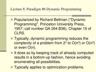
Lecture 8. Paradigm #6 Dynamic Programming. Popularized by Richard Bellman ("Dynamic Programming", Princeton University Press, 1957; call number QA 264.B36). Chapter 15 of CLRS. Typically, dynamic programming reduces the complexity of a problem from 2 n to O(n 3 ) or O(n 2 ) or even O(n).

Lecture 8. Paradigm #6 Dynamic Programming
E N D
Presentation Transcript
Lecture 8. Paradigm #6 Dynamic Programming • Popularized by Richard Bellman ("Dynamic Programming", Princeton University Press, 1957; call number QA 264.B36). Chapter 15 of CLRS. • Typically, dynamic programming reduces the complexity of a problem from 2n to O(n3) or O(n2) or even O(n). • It does so by keeping track of already computed results in a bottom-up fashion, hence avoiding enumerating all possibilities. • Typically applies to optimization problems.
Example 1. Efficient multiplication of matrices (Section 15.2 of CLRS.) • Suppose we are given the following 3 matrices: • M1 10 x 100 • M2 100 x 5 • M3 5 x 50 • There are two ways to compute M1*M2*M3: M1 (M2 M3) or (M1 M2) M3 • Since the cost of multiplying a p x q matrix by a q x r matrix is pqr multiplications, the cost of M1 (M2 M3) is 100 x 5 x 50 + 10 x 100 x 50 = 75,000 multiplications, while the cost of (M1 M2) M3 is 10 x 100 x 5 + 10 x 5 x 50 = 7,500 multiplications: a difference of a factor of 10.
Naïve approach • We could enumerate all possibilities, and then take the minimum. How many possibilities are there? • The LAST multiplication performed is either M1*(M2 ... Mn), or (M1 M2)*(M3 ... Mn), or ... (M1 M2 ...)(Mn). Therefore, W(n), the number of ways to compute M1 M2 ... Mn, satisfies the following recurrence: W(n) = Σ1 ≤ k < n W(k)W(n-k) --- Catalan number • Now it can be proved by induction that W(n) = (2n-2 choose n-1)/n. Using Stirling's approximation, which says that n! = √(2πn) nn e-n (1 + o(1)), we have (2n choose n) ~ 22n/√(π n), • We conclude that W(n) ~ 4n n-3/2, which means our naive approach will simply take too long (about 1010 steps when n = 20).
Dynamic Programming approach • Let’s avoid all the re-computation of the recursive approach. • Observe: Suppose the optimal method to compute M1 M2 ... Mn were to first compute M1 M2 ... Mk (in some order), then compute Mk+1 ... Mn (in some order), and then multiply these together. Then the method used for M1 M2 ... Mkmust be optimal, for otherwise we could substitute a superior method and improve the optimal method. Similarly, the method used to compute Mk+1 ... Mn must also be optimal. The only thing left to do is to find the best possible k, and there are only n choices for that. • Letting m[i,j] represent the optimal cost for computing the product Mi ... Mj, we see that m[i,j] = min { m[i,k] + m[k+1,j] + p[i-1]p[k]p[j] }, i ≤ k < j • k represents the optimal place to break the product Mi ... Mj into two pieces. Here p is an array such that M1 is of dimension p[0] × p[1], M2 is of dimension p[1] × p[2], ... etc.
Implementing it --- O(n3) time • Like the Fibonacci number example, we cannot implement this by recursion. It will be exponential time. • MATRIX-MULT-ORDER(p) /* p[0..n] is an array holding the dimensions of the matrices; matrix i has dimension p[i-1] x p[i] */ for i := 1 to n do m[i,i] := 0 for d := 1 to n-1 do // d is the size of the sub-problem. for i := 1 to n-d do j := i+d m[i,j] := infinity; for k := i to j-1 do q := m[i,k] + m[k+1,j] + p[i-1]*p[k]*p[j] if q < m[i,j] then m[i,j] := q s[i,j] := k // optimal position for breaking m[i,j] return(m,s)
Actually multiply the matrices • We have stored the break points k’s in the array s. s[i,j] represents the optimal place to break the product Mi ... Mj. We can use s now to multiply the matrices: • MATRIX-MULT(M, s, i, j) /* Given the matrix s calculated by MATRIX-MULT-ORDER. The list of matrices M = [M1, M2, ... , Mn]. Starting and finishing indices i and j. This routine computes the product Mi ... Mj using the optimal method */ if j > i then X := MATRIX-MULT(M, s, i, s[i,j]); Y := MATRIX-MULT(M, s, s[i,j]+1, j); return(X*Y); else return(Mi)
Longest Common Subsequence (LCS) Application: comparison of two DNA strings Ex: X= {A B C B D A B }, Y= {B D C A B A} Longest Common Subsequence: X = A BCB D A B Y = B D C A BA Brute force algorithm would compare each subsequence of X with the symbols in Y
LCS Algorithm • if |X| = m, |Y| = n, then there are 2m subsequences of x; we must compare each with Y (n comparisons) • So the running time of the brute-force algorithm is O(n 2m) • Notice that the LCS problem has optimal substructure: solutions of subproblems are parts of the final solution – often, this is when you can use dynamic programming. • Subproblems: “find LCS of pairs of prefixes of X and Y”
LCS Algorithm • First we’ll find the length of LCS. Later we’ll modify the algorithm to find LCS itself. • Let Xi, Yj be the prefixes of X and Y of length i and j respectively • Let c[i,j] be the length of LCS of Xi and Yj • Then the length of LCS of X and Y will be c[m,n]
LCS recursive solution • We start with i = j = 0 (empty substrings of x and y) • Since X0 and Y0 are empty strings, their LCS is always empty (i.e. c[0,0] = 0) • LCS of empty string and any other string is empty, so for every i and j: c[0, j] = c[i,0] = 0
LCS recursive solution • When we calculate c[i,j], we consider two cases: • First case:x[i]=y[j]: one more symbol in strings X and Y matches, so the length of LCS Xi and Yjequals to the length of LCS of smaller strings Xi-1 and Yi-1 , plus 1
LCS recursive solution • Second case:x[i] != y[j] • As symbols don’t match, our solution is not improved, and the length of LCS(Xi , Yj) is the same as before, we take the maximum of LCS(Xi, Yj-1) and LCS(Xi-1,Yj) Think: Why can’t we just take the length of LCS(Xi-1, Yj-1) ?
LCS Length Algorithm LCS-Length(X, Y) 1. m = length(X) // get the # of symbols in X 2. n = length(Y) // get the # of symbols in Y 3. for i = 1 to m c[i,0] = 0 // special case: Y0 4. for j = 1 to n c[0,j] = 0 // special case: X0 5. for i = 1 to m // for all Xi 6. for j = 1 to n // for all Yj 7. if ( Xi == Yj ) 8. c[i,j] = c[i-1,j-1] + 1 9. else c[i,j] = max( c[i-1,j], c[i,j-1] ) 10. return c
LCS Example We’ll see how LCS algorithm works on the following example: • X = ABCB • Y = BDCAB LCS(X, Y) = BCB X = A BCB Y = B D C A B
LCS Example (0) ABCB BDCAB j 0 1 2 3 4 5 i Yj B D C A B Xi 0 A 1 B 2 3 C 4 B X = ABCB; m = |X| = 4 Y = BDCAB; n = |Y| = 5 Allocate array c[5,4]
LCS Example (1) ABCB BDCAB j 0 1 2 3 4 5 i Yj B D C A B Xi 0 0 0 0 0 0 0 A 1 0 B 2 0 3 C 0 4 B 0 for i = 1 to m c[i,0] = 0 for j = 1 to n c[0,j] = 0
LCS Example (2) ABCB BDCAB j 0 1 2 3 4 5 i Yj B D C A B Xi 0 0 0 0 0 0 0 A 1 0 0 B 2 0 3 C 0 4 B 0 if ( Xi == Yj ) c[i,j] = c[i-1,j-1] + 1 else c[i,j] = max( c[i-1,j], c[i,j-1] )
LCS Example (3) ABCB BDCAB j 0 1 2 3 4 5 i Yj B D C A B Xi 0 0 0 0 0 0 0 A 1 0 0 0 0 B 2 0 3 C 0 4 B 0 if ( Xi == Yj ) c[i,j] = c[i-1,j-1] + 1 else c[i,j] = max( c[i-1,j], c[i,j-1] )
LCS Example (4) ABCB BDCAB j 0 1 2 3 4 5 i Yj B D C A B Xi 0 0 0 0 0 0 0 A 1 0 0 0 0 1 B 2 0 3 C 0 4 B 0 if ( Xi == Yj ) c[i,j] = c[i-1,j-1] + 1 else c[i,j] = max( c[i-1,j], c[i,j-1] )
LCS Example (5) ABCB BDCAB j 0 1 2 3 4 5 i Yj B D C A B Xi 0 0 0 0 0 0 0 A 1 0 0 0 0 1 1 B 2 0 3 C 0 4 B 0 if ( Xi == Yj ) c[i,j] = c[i-1,j-1] + 1 else c[i,j] = max( c[i-1,j], c[i,j-1] )
LCS Example (6) ABCB BDCAB j 0 1 2 3 4 5 i Yj B D C A B Xi 0 0 0 0 0 0 0 A 1 0 0 0 0 1 1 B 2 0 1 3 C 0 4 B 0 if ( Xi == Yj ) c[i,j] = c[i-1,j-1] + 1 else c[i,j] = max( c[i-1,j], c[i,j-1] )
LCS Example (7) ABCB BDCAB j 0 1 2 3 4 5 i Yj B D C A B Xi 0 0 0 0 0 0 0 A 1 0 0 0 0 1 1 B 2 0 1 1 1 1 3 C 0 4 B 0 if ( Xi == Yj ) c[i,j] = c[i-1,j-1] + 1 else c[i,j] = max( c[i-1,j], c[i,j-1] )
LCS Example (8) ABCB BDCAB j 0 1 2 3 4 5 i Yj B D C A B Xi 0 0 0 0 0 0 0 A 1 0 0 0 0 1 1 B 2 0 1 1 1 1 2 3 C 0 4 B 0 if ( Xi == Yj ) c[i,j] = c[i-1,j-1] + 1 else c[i,j] = max( c[i-1,j], c[i,j-1] )
LCS Example (10) ABCB BDCAB j 0 1 2 3 4 5 i Yj B D C A B Xi 0 0 0 0 0 0 0 A 1 0 0 0 0 1 1 B 2 0 1 1 1 1 2 3 C 0 1 1 4 B 0 if ( Xi == Yj ) c[i,j] = c[i-1,j-1] + 1 else c[i,j] = max( c[i-1,j], c[i,j-1] )
LCS Example (11) ABCB BDCAB j 0 1 2 3 4 5 i Yj B D C A B Xi 0 0 0 0 0 0 0 A 1 0 0 0 0 1 1 B 2 0 1 1 1 1 2 3 C 0 1 1 2 4 B 0 if ( Xi == Yj ) c[i,j] = c[i-1,j-1] + 1 else c[i,j] = max( c[i-1,j], c[i,j-1] )
LCS Example (12) ABCB BDCAB j 0 1 2 3 4 5 i Yj B D C A B Xi 0 0 0 0 0 0 0 A 1 0 0 0 0 1 1 B 2 0 1 1 1 1 2 3 C 0 1 1 2 2 2 4 B 0 if ( Xi == Yj ) c[i,j] = c[i-1,j-1] + 1 else c[i,j] = max( c[i-1,j], c[i,j-1] )
LCS Example (13) ABCB BDCAB j 0 1 2 3 4 5 i Yj B D C A B Xi 0 0 0 0 0 0 0 A 1 0 0 0 0 1 1 B 2 0 1 1 1 1 2 3 C 0 1 1 2 2 2 4 B 0 1 if ( Xi == Yj ) c[i,j] = c[i-1,j-1] + 1 else c[i,j] = max( c[i-1,j], c[i,j-1] )
LCS Example (14) ABCB BDCAB j 0 1 2 34 5 i Yj B D C A B Xi 0 0 0 0 0 0 0 A 1 0 0 0 0 1 1 B 2 0 1 1 1 1 2 3 C 0 1 1 2 2 2 4 B 0 1 1 2 2 if ( Xi == Yj ) c[i,j] = c[i-1,j-1] + 1 else c[i,j] = max( c[i-1,j], c[i,j-1] )
LCS Example (15) ABCB BDCAB j 0 1 2 3 4 5 i Yj B D C A B Xi 0 0 0 0 0 0 0 A 1 0 0 0 0 1 1 B 2 0 1 1 1 1 2 3 C 0 1 1 2 2 2 3 4 B 0 1 1 2 2 if ( Xi == Yj ) c[i,j] = c[i-1,j-1] + 1 else c[i,j] = max( c[i-1,j], c[i,j-1] )
LCS Algorithm Running Time • LCS algorithm calculates the values of each entry of the array c[m,n] • So what is the running time? O(m*n) since each c[i,j] is calculated in constant time, and there are m*n elements in the array
How to find actual LCS • So far, we have just found the length of LCS, but not LCS itself. • We want to modify this algorithm to make it output Longest Common Subsequence of X and Y Each c[i,j] depends on c[i-1,j] and c[i,j-1] or c[i-1, j-1] For each c[i,j] we can say how it was acquired: For example, here c[i,j] = c[i-1,j-1] +1 = 2+1=3 2 2 2 3
How to find actual LCS - continued • Remember that • So we can start from c[m,n] and go backwards • Whenever c[i,j] = c[i-1, j-1]+1, remember x[i] (because x[i] is a part of LCS) • When i=0 or j=0 (i.e. we reached the beginning), output remembered letters in reverse order
Finding LCS j 0 1 2 3 4 5 i Yj B D C A B Xi 0 0 0 0 0 0 0 A 1 0 0 0 0 1 1 B 2 0 1 1 1 1 2 3 C 0 1 1 2 2 2 3 4 B 0 1 1 2 2
Finding LCS (2) j 0 1 2 3 4 5 i Yj B D C A B Xi 0 0 0 0 0 0 0 A 1 0 0 0 0 1 1 B 2 0 1 1 1 1 2 3 C 0 1 1 2 2 2 3 4 B 0 1 1 2 2 LCS (reversed order): B C B B C B (this string turned out to be a palindrome) LCS (straight order):
If we have time, we will do some exercises in class: • Edit distance: Given two text strings A of length n and B of length m, you want to transform A into B with a minimum number of operations of the following types: delete a character from A, insert a character into A, or change some character in A into a new character. The minimal number of such operations required to transform A into B is called the edit distance between A and B. • Balanced Partition: Given a set of n integers each in the range 0 ... K. Partition these integers into two subsets such that you minimize |S1 - S2|, where S1 and S2 denote the sums of the elements in each of the two subsets.