Unit 4: Dynamic Programming
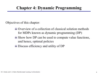
Unit 4: Dynamic Programming. Course contents: Assembly-line scheduling Rod cutting Matrix-chain multiplication Longest common subsequence Optimal binary search trees Applications: optimal polygon triangulation, flip-chip routing, technology mapping for logic synthesis Reading: Chapter 15.

Unit 4: Dynamic Programming
E N D
Presentation Transcript
Unit 4: Dynamic Programming • Course contents: • Assembly-line scheduling • Rod cutting • Matrix-chain multiplication • Longest common subsequence • Optimal binary search trees • Applications: optimal polygon triangulation, flip-chip routing, technology mapping for logic synthesis • Reading: • Chapter 15 Spring 2013 1
Dynamic Programming (DP) vs. Divide-and-Conquer • Both solve problems by combining the solutions to subproblems. • Divide-and-conquer algorithms • Partition a problem into independent subproblems, solve the subproblems recursively, and then combine their solutions to solve the original problem. • Inefficient if they solve the same subproblem more than once. • Dynamic programming (DP) • Applicable when the subproblems are not independent. • DP solves each subproblem just once. Spring 2013 2
Assembly-line Scheduling S1,n S1,3 S1,n-1 station S1,1 S1,2 a1,3 a1,1 a1,2 a1,n-1 line 1 a1,n e1 x1 t1,2 t1,1 t1,n-1 auto exits chassis enters t2,2 t2,1 t2,n-1 x2 e2 a2,1 a2,3 a2,n-1 a2,2 a2,n line 2 S2,n S2,3 S2,n-1 station S2,1 S2,2 • An auto chassis enters each assembly line, has parts added at stations, and a finished auto exits at the end of the line. • Si,j: the jth station on line i • ai,j: the assembly time required at station Si,j • ti,j: transfer time from station Si,j to the j+1 station of the other line. • ei (xi): time to enter (exit) line i Spring 2013 3
Optimal Substructure S1,n S1,3 S1,n-1 S1,1 S1,2 a1,3 a1,1 a1,2 a1,n-1 a1,n line 1 e1 x1 t1,2 t1,1 t1,n-1 auto exits chassis enters t2,2 t2,1 t2,n-1 x2 e2 a2,1 a2,3 a2,n-1 a2,2 a2,n line 2 S2,n S2,n-1 S2,3 S2,1 S2,2 • Objective: Determine the stations to choose to minimize the total manufacturing time for one auto. • Brute force: (2n), why? • The problem is linearly ordered and cannot be rearranged => Dynamic programming? • Optimal substructure: If the fastest way through station Si,j is through S1,j-1, then the chassis must have taken a fastest way from the starting point through S1,j-1. Spring 2013 4
Overlapping Subproblem: Recurrence S1,n S1,3 S1,n-1 S1,1 S1,2 a1,3 a1,1 a1,2 a1,n-1 a1,n line 1 e1 x1 t1,2 t1,1 t1,n-1 auto exits chassis enters t2,2 t2,1 t2,n-1 x2 e2 a2,1 a2,3 a2,n-1 a2,2 a2,n line 2 S2,n S2,n-1 S2,3 S2,1 S2,2 • Overlapping subproblem: The fastest way through station S1,j is either through S1,j-1 and thenS1,j , or through S2,j-1 and then transfer to line 1 and through S1,j. • fi[j]: fastest time from the starting point through Si,j • The fastest time all the way through the factory f* = min(f1[n] + x1, f2[n] + x2) Spring 2013 5
Computing the Fastest Time Fastest-Way(a, t, e, x, n) 1. f1[1]=e1 + a1,1 2. f2[1]=e2 + a2,1 3.forj= 2 ton 4. iff1[j-1] + a1,j f2[j-1] + t2,j -1 + a1,j 5. f1[j]=f1[j-1] + a1,j 6. l1[j] =1 7. elsef1[j]=f2[j-1] + t2,j -1 + a1,j 8. l1[j] =2 9. iff2[j-1] + a2,j f1[j-1] + t1,j -1 + a2,j 10. f2[j]=f2[j-1] + a2,j 11. l2[j] =2 12. elsef2[j]=f1[j-1] + t1,j -1 + a2,j 13. l2[j] =1 14. iff1[n] + x1f2[n] + x2 15. f* =f1[n] + x1 16. l* = 1 17. elsef* =f2[n] + x2 18. l* = 2 • li[j]: The line number whose station j-1 is used in a fastest way through Si,j Running time? Linear time!! Spring 2013 6
Constructing the Fastest Way S1,4 S1,6 S1,3 S1,5 S1,1 S1,2 3 4 7 9 8 4 line 1 2 3 3 3 2 1 4 auto exits chassis enters 1 2 2 2 1 2 4 8 4 6 5 5 7 line 2 S2,4 S2,6 S2,5 S2,3 S2,1 S2,2 Print-Station(l, n) 1. i =l* 2. Print “line” i “, station “ n 3. forj= n downto2 4. i =li[j] 5. Print “line “ i “, station “ j-1 line 1, station 6 line 2, station 5 line 2, station 4 line 1, station 3 line 2, station 2 line 1, station 1 Spring 2013 7
An Example S1,4 S1,6 S1,3 S1,5 S1,1 S1,2 3 4 7 9 8 4 line 1 2 3 3 3 2 1 4 auto exits chassis enters 1 2 2 2 1 2 4 8 4 6 5 5 7 line 2 S2,4 S2,6 S2,5 S2,3 S2,1 S2,2 f1[j] f* = 38 f2[j] 1 2 3 4 5 j 6 l1[j] l* = 1 l2[j] Spring 2013 8
Dynamic Programming (DP) • Typically apply to optimization problem. • Generic approach • Calculate the solutions to all subproblems. • Proceed computation from the small subproblems to larger subproblems. • Compute a subproblem based on previously computed results for smaller subproblems. • Store the solution to a subproblem in a table and never recompute. • Development of a DP • Characterize the structure of an optimal solution. • Recursively define the value of an optimal solution. • Compute the value of an optimal solution bottom-up. • Construct an optimal solution from computed information (omitted if only the optimal value is required). Spring 2013 9
When to Use Dynamic Programming (DP) • DP computes recurrence efficiently by storing partial results efficient only when the number of partial results is small. • Hopeless configurations:n! permutations of an n-element set, 2n subsets of an n-element set, etc. • Promising configurations: contiguous substrings of an n-character string, n(n+1)/2 possible subtrees of a binary search tree, etc. • DP works best on objects that are linearly ordered and cannot be rearranged!! • Linear assembly lines, matrices in a chain, characters in a string, points around the boundary of a polygon, points on a line/circle, the left-to-right order of leaves in a search tree, etc. • Objects are ordered left-to-right Smell DP? Spring 2013 10
Rod Cutting Cut steel rods into pieces to maximize the revenue Each cut is free; rod lengths are integral numbers. Input: A length n and table of prices pi, for i = 1, 2, …, n. Output: The maximum revenue obtainable for rods whose lengths sum to n, computed as the sum of the prices for the individual rods. 8 1 5 9 5 1 5 8 5 length i = 4 1 5 1 1 1 1 1 1 1 1 1 5 5 max revenue r4 = 5+5 =10 Objectsare linearly ordered (and cannot be rearranged)?? Spring 2013 11
Optimal Rod Cutting • If pn is large enough, an optimal solution might require no cuts, i.e., just leave the rod as n unit long. • Solution for the maximum revenue ri of length i r1 = 1 from solution 1 = 1 (no cuts) r2 = 5 from solution 2 = 2 (no cuts) r3 = 8 from solution 3 = 3 (no cuts) r4 = 10 from solution 4 = 2 + 2 r5 = 13 from solution 5 = 2 + 3 r6 = 17 from solution 6 = 6 (no cuts) r7 = 18 from solution 7 = 1 + 6 or 7 = 2 + 2 + 3 r8 = 22 from solution 8 = 2 + 6 Spring 2013 12
Optimal Substructure • Optimal substructure: To solve the original problem, solve subproblems on smaller sizes. The optimal solution to the original problem incorporates optimal solutions to the subproblems. • We may solve the subproblems independently. • After making a cut, we have two subproblems. • Max revenue r7: r7 = 18 = r4 + r3 = (r2 + r2) + r3 or r1 + r6 • Decomposition with only one subproblem: Some cut gives a first piece of length i on the left and a remaining piece of length n - i on the right. Spring 2013 13
Recursive Top-Down “Solution” • Inefficient solution: Cut-Rod calls itself repeatedly, even on subproblems it has already solved!! Cut-Rod(p, n) 1. ifn == 0 2. return 0 3.q = - ∞ 4. fori= 1 ton 5. q = max(q, p[i] + Cut-Rod(p, n - i)) 6. returnq Cut-Rod(p, 4) Cut-Rod(p, 3) Cut-Rod(p, 1) T(n) = 2n Overlapping subproblems? Cut-Rod(p, 0) Spring 2013 14
Top-Down DP Cut-Rod with Memoization • Complexity: O(n2) time • Solve each subproblem just once, and solves subproblems for sizes 0,1, …, n. To solve a subproblem of size n, the forloop iterates n times. Memoized-Cut-Rod(p, n) 1. let r[0..n] be a new array 2.fori= 0 to n 3. r[i] = - 4.returnMemoized-Cut-Rod -Aux(p, n, r) Memoized-Cut-Rod-Aux(p, n, r) 1. ifr[n] ≥ 0 2. returnr[n] 3. ifn == 0 4. q = 0 5. else q = - ∞ 6. fori= 1 ton 7. q = max(q, p[i] + Memoized-Cut-Rod -Aux(p, n-i, r)) 8. r[n] = q 9. returnq // Each overlapping subproblem // is solved just once!! Spring 2013 15
Bottom-Up DP Cut-Rod • Complexity: O(n2) time • Sort the subproblems by size and solve smaller ones first. • When solving a subproblem, have already solved the smaller subproblems we need. Bottom-Up-Cut-Rod(p, n) 1. let r[0..n] be a new array 2. r[0] = 0 3. forj= 1 ton 4. q = - ∞ 5. fori= 1 toj 6. q = max(q, p[i] + r[j – i]) 7. r[j] = q 8. returnr[n] Spring 2013 16
Bottom-Up DP with Solution Construction Extended-Bottom-Up-Cut-Rod(p, n) 1. let r[0..n] and s[0..n] be new arrays 2. r[0] = 0 3. forj= 1 ton 4. q = - ∞ 5. fori= 1 toj 6. ifq < p[i] + r[j – i] 7. q = p[i] + r[j – i] 8. s[j] = i 9. r[j] = q 10. returnr and s • Extend the bottom-up approach to record not just optimal values, but optimal choices. • Saves the first cut made in an optimal solution for a problem of size i in s[i]. 5 5 5 5 Print-Cut-Rod-Solution(p, n) 1. (r, s) = Extended-Bottom-Up-Cut-Rod(p, n) 2. while n > 0 3. print s[n] 4. n = n – s[n] 17 1 Spring 2013 17
DP Example: Matrix-Chain Multiplication • If A is a pxqmatrix and B a qxrmatrix, then C = AB is a pxrmatrix time complexity: O(pqr). Matrix-Multiply(A, B) 1. ifA.columns≠ B.rows 2. error “incompatible dimensions” 3.elselet C be a new A.rows * B.columns matrix 4. fori= 1 toA.rows 5. forj=1toB.columns 6. cij = 0 7. fork = 1to A.columns 8. cij = cij + aikbkj 9. returnC Spring 2013 18
DP Example: Matrix-Chain Multiplication • The matrix-chain multiplication problem • Input: Given a chain <A1, A2, …, An> of n matrices, matrix Aihas dimension pi-1xpi • Objective: Parenthesize the product A1A2 … An to minimize the number of scalar multiplications • Exp: dimensions: A1: 4 x 2; A2: 2 x 5; A3: 5 x 1 (A1A2)A3: total multiplications = 4 x2 x5 + 4 x5 x1 = 60 A1(A2A3): total multiplications = 2 x5 x1 + 4 x2 x1 = 18 • So the order of multiplications can make a big difference! Spring 2013 19
Matrix-Chain Multiplication: Brute Force • A = A1A2 … An: How to evaluate A using the minimum number of multiplications? • Brute force: check all possible orders? • P(n): number of ways to multiply n matrices. • , exponential in n. • Any efficient solution? • The matrix chainis linearly ordered and cannot be rearranged!! • Smell Dynamic programming? Spring 2013 20
Matrix-Chain Multiplication • m[i, j]: minimum number of multiplications to compute matrix Ai..j = AiAi+1 … Aj, 1 i j n. • m[1, n]: the cheapest cost to compute A1..n. • Applicability of dynamic programming • Optimal substructure: an optimal solution contains within its optimal solutions to subproblems. • Overlapping subproblem: a recursive algorithm revisits the same problem over and over again; only (n2) subproblems. matrix Aihas dimension pi-1xpi Spring 2013 21
Bottom-Up DP Matrix-Chain Order Matrix-Chain-Order(p) 1. n =p.length – 1 2. Let m[1..n, 1..n] and s[1..n-1, 2..n] be new tables 3. fori= 1 ton 4. m[i, i] = 0 5.forl= 2 ton // l is the chain length 6. fori= 1 ton – l +1 7. j=i + l -1 8. m[i, j] = 9. fork=i toj -1 10. q=m[i, k] + m[k+1, j] + pi-1pkpj 11. if q < m[i, j] 12. m[i, j] =q 13. s[i, j] =k 14. returnm and s Aidimension pi-1xpi s Spring 2013 22
Constructing an Optimal Solution • s[i, j]: value of k such that the optimal parenthesization of AiAi+1 … Aj splits between Ak and Ak+1 • Optimal matrix A1..n multiplication: A1..s[1, n]As[1, n] + 1..n • Exp: call Print-Optimal-Parens(s, 1, 6): ((A1 (A2A3))((A4A5) A6)) Print-Optimal-Parens(s, i, j) 1. ifi == j 2. print “A”i 3. else print “(“ 4. Print-Optimal-Parens(s, i, s[i, j]) 5. Print-Optimal-Parens(s, s[i, j] + 1, j) 6. print “)“ s 0 Spring 2013 23
Top-Down, Recursive Matrix-Chain Order • Time complexity: (2n) (T(n) > (T(k)+T(n-k)+1)). Recursive-Matrix-Chain(p, i, j) 1. ifi == j 2. return 0 3. m[i, j] = 4. fork=itoj -1 5 q= Recursive-Matrix-Chain(p,i, k) + Recursive-Matrix-Chain(p, k+1, j) + pi-1pkpj 6. if q < m[i, j] 7. m[i, j] =q 8. returnm[i, j] Spring 2013 24
Top-Down DP Matrix-Chain Order (Memoization) • Complexity: O(n2) space for m[] matrix and O(n3) time to fill in O(n2) entries (each takes O(n) time) Memoized-Matrix-Chain(p) 1. n =p.length - 1 2. let m[1..n, 1..n] be a new table 2. fori= 1 to n 3. forj =iton 4. m[i, j] = 5. return Lookup-Chain(m, p,1,n) Lookup-Chain(m, p, i, j) 1. if m[i, j] < 2. return m[i, j] 3. if i == j 4. m[ i, j] = 0 5. else fork=itoj -1 6. q= Lookup-Chain(m, p, i, k) + Lookup-Chain(m, p, k+1, j) + pi-1pkpj 7. if q < m[i, j] 8. m[i, j] = q 9. return m[i, j] Spring 2013 25
Two Approaches to DP • Bottom-up iterative approach • Start with recursive divide-and-conquer algorithm. • Find the dependencies between the subproblems (whose solutions are needed for computing a subproblem). • Solve the subproblems in the correct order. • Top-down recursive approach (memoization) • Start with recursive divide-and-conquer algorithm. • Keep top-down approach of original algorithms. • Save solutions to subproblems in a table (possibly a lot of storage). • Recurse only on a subproblem if the solution is not already available in the table. • If all subproblems must be solved at least once, bottom-up DP is better due to less overhead for recursion and for maintaining tables. • If many subproblems need not be solved, top-down DP is better since it computes only those required. Spring 2013 26
Longest Common Subsequence • Problem: Given X = <x1, x2, …, xm> and Y = <y1, y2, …, yn>, find the longest common subsequence (LCS)of X and Y. • Exp:X = <a, b, c, b, d, a, b> and Y = <b, d,c, a, b, a> LCS = <b, c, b, a> (also, LCS = <b, d, a, b>). • Exp: DNA sequencing: • S1 = ACCGGTCGAGATGCAG; S2 = GTCGTTCGGAATGCAT; LCS S3 = CGTCGGATGCA • Brute-force method: • Enumerate all subsequences of X and check if they appear in Y. • Each subsequence of X corresponds to a subset of the indices {1, 2, …, m} of the elements of X. • There are 2m subsequences of X. Why? Spring 2013 27
Optimal Substructure for LCS • Let X = <x1, x2, …, xm> and Y= <y1, y2, …, yn> be sequences, and Z = <z1, z2, …, zk> be LCS of X and Y. • If xm = yn, then zk = xm = ynand Zk-1 is an LCS of Xm-1 and Yn-1. • If xm≠ yn, then zk≠xmimplies Z is an LCS of Xm-1 and Y. • If xm≠ yn, then zk≠ynimplies Z is an LCS of X and Yn-1. • c[i, j]: length of the LCS of Xi and Yj • c[m, n]: length of LCS of X and Y • Basis: c[0, j] = 0 and c[i, 0] = 0 Spring 2013 28
Top-Down DP for LCS • c[i, j]: length of the LCS of Xi and Yj, where Xi = <x1, x2, …, xi> and Yj=<y1, y2, …, yj>. • c[m, n]: LCS of X and Y. • Basis: c[0, j] = 0 and c[i, 0] = 0. • The top-down dynamic programming: initialize c[i, 0] = c[0, j] = 0, c[i, j] = NIL TD-LCS(i, j) 1.if c[i,j] == NIL 2. ifxi == yj 3. c[i, j] = TD-LCS(i-1, j-1) + 1 4. elsec[i, j] = max(TD-LCS(i, j-1), TD-LCS(i-1, j)) 5. returnc[i, j] Spring 2013 29
Bottom-Up DP for LCS LCS-Length(X,Y) 1. m=X.length 2. n=Y.length 3. let b[1..m, 1..n] and c[0..m, 0..n] be new tables 4. fori= 1 tom 5. c[i, 0] = 0 6. forj= 0 ton 7. c[0, j] = 0 8. fori= 1 tom 9. forj= 1 ton 10. ifxi == yj 11. c[i, j] =c[i-1, j-1]+1 12. b[i, j] = “↖” 13. elseifc[i-1,j] c[i, j-1] 14. c[i,j] = c[i-1, j] 15. b[i, j] = `` '' 16. elsec[i, j] =c[i, j-1] 17. b[i, j] = “ “ 18. returnc and b • Find the right order to solve the subproblems • To compute c[i, j], we need c[i-1, j-1], c[i-1, j], and c[i, j-1] • b[i, j]: points to the table entry w.r.t. the optimal subproblem solution chosen when computing c[i, j] Spring 2013 30
Example of LCS • LCS time and space complexity: O(mn). • X = <A, B, C, B, D, A, B> and Y = <B, D, C, A, B, A> LCS = <B, C, B, A>. Spring 2013 31
Constructing an LCS • Trace back from b[m, n] to b[1, 1], following the arrows: O(m+n) time. Print-LCS(b, X, i, j) 1. ifi == 0 or j == 0 2. return 3. ifb[i, j] == “↖ “ 4. Print-LCS(b, X, i-1, j-1) 5. print xi 6. elseifb[i, j] == “ “ 7. Print-LCS(b, X, i -1, j) 8. elsePrint-LCS(b, X, i, j-1) Spring 2013 32
Optimal Binary Search Tree k2 k2 k1 k5 k1 k4 d5 k4 k3 k5 d1 d0 d0 d1 d4 k3 d5 d2 d3 d4 d3 d2 • Given a sequence K = <k1, k2, …, kn> of n distinct keys in sorted order (k1 < k2 < … < kn) and a set of probabilities P = <p1, p2, …, pn> for searching the keys in K and Q = <q0, q1, q2, …, qn> for unsuccessful searches (corresponding to D = <d0, d1, d2, …, dn> of n+1distinct dummy keys with di representing all values between ki and ki+1), construct a binary search tree whose expected search cost is smallest. p2 p1 p4 p5 p3 q1 q0 q5 q2 q4 q3 Spring 2013 33
An Example 0.10×1 (depth 0) 0.15×2 0.10×2 0.20×3 k2 k2 k1 k5 k1 k4 0.10×4 Cost = 2.80 d5 k4 k3 k5 d1 d0 d0 d1 d4 k3 d5 d2 d3 d4 d3 d2 Cost = 2.75 Optimal!! Spring 2013 34
Optimal Substructure k2 k1 k5 d5 k4 d1 d0 d4 k3 d3 d2 • If an optimal binary search tree T has a subtree T’ containing keys ki, …, kj, then this subtree T’ must be optimal as well for the subproblem with keys ki, …, kj and dummy keys di-1, …, dj. • Given keys ki, …, kj with kr (irj) as the root, the left subtree contains the keys ki, …, kr-1 (and dummy keys di-1, …, dr-1) and the right subtree contains the keys kr+1, …, kj (and dummy keys dr, …, dj). • For the subtree with keys ki, …, kj with root ki, the left subtree contains keys ki, .., ki-1 (no key) with the dummy key di-1. Spring 2013 35
Overlapping Subproblem: Recurrence Node depths increase by 1 after merging two subtrees, and so do the costs 0.10×1 k4 k3 k5 0.20×2 0.10×3 d5 d2 d3 d4 • e[i, j] : expected cost of searching an optimal binary search tree containing the keys ki, …, kj. • Want to find e[1, n]. • e[i, i -1] = qi-1 (only the dummy key di-1). • If kr (irj) is the root of an optimal subtree containing keys ki, …, kj and letthen e[i, j] = pr+ (e[i, r-1] + w(i, r-1)) + (e[r+1, j] +w(r+1, j)) = e[i, r-1] + e[r+1, j] + w(i, j) • Recurrence: Spring 2013 36
Computing the Optimal Cost 0.70 0.10 0.05 0.05 1.75 0.05 0.05 0.30 0.50 2.75 0.60 0.45 0.40 0.10 1.30 0.90 2.00 0.25 1.25 0.90 1.20 e 5 1 4 2 3 i j 3 2 4 1 5 0 6 • Need a table e[1..n+1, 0..n] for e[i, j] (why e[1, 0] and e[n+1, n]?) • Apply the recurrence to compute w(i, j) (why?) k4 k3 k5 Optimal-BST(p, q, n) 1. let e[1..n+1, 0..n], w[1..n+1, 0..n], and root[1..n, 1..n] be new tables 2. fori= 1 ton + 1 3. e[i, i-1] =qi-1 4. w[i, i-1] =qi-1 5.forl= 1 ton 6. fori= 1 ton – l + 1 7. j=i + l -1 8. e[i, j] = 9. w[i, j] =w[i, j-1] + pj+ qj 10. forr=i toj 11. t=e[i, r-1] + e[r+1, j] + w[i, j] 12. if t < e[i, j] 13. e[i, j] =t 14. root[i, j] =r 15. returne and root d5 d2 d3 d4 • root[i, j] : index r for which kr is the root of an optimal search tree containing keys ki, …, kj. Spring 2013 37
Example w e 1 5 1 5 i j 2 4 2 4 4 5 4 2 1 0.05 0.90 2.00 0.10 1.75 1.20 0.05 2.75 0.50 0.05 0.90 0.40 0.60 0.70 0.25 0.05 0.10 1.30 1.25 0.30 0.05 0.45 0.70 1.00 0.80 0.30 0.60 0.05 0.50 0.10 0.45 0.50 0.35 0.30 0.20 0.25 0.55 0.35 0.15 0.10 0.05 0.05 4 2 2 5 2 1 5 2 2 3 i j 3 3 3 3 4 2 4 2 1 5 root 1 5 0 6 5 1 0 6 4 2 j i 3 3 k2 2 4 k1 k5 1 5 d5 k4 d1 d0 d4 k3 d3 d2 e[1, 1] = e[1, 0] + e[2, 1] + w(1,1) = 0.05 + 0.10 + 0.3 = 0.45 e[1, 5] = e[1, 1] + e[3, 5] + w(1,5) = 0.45 + 1.30 + 1.00 = 2.75 Spring 2013 38
Appendix A: Optimal Polygon Triangulation • Terminology: polygon, interior, exterior, boundary, convex polygon, triangulation? • The Optimal Polygon Triangulation Problem: Given a convex polygon P = <v0, v1, …, vn-1> and a weight function w defined on triangles, find a triangulation that minimizes w(). • One possible weight function on triangle: w(vivjvk)=|vivj| + |vjvk| + |vkvi|, where |vivj| is the Euclidean distance from vi to vj. Spring 2013 39
Optimal Polygon Triangulation (cont'd) • Correspondence between full parenthesization, full binary tree (parse tree), and triangulation • full parenthesization full binary tree • full binary tree (n-1 leaves) triangulation (n sides) • t[i, j]: weight of an optimal triangulation of polygon <vi-1, vi, …, vj>. Spring 2013 40
Pseudocode: Optimal Polygon Triangulation • Matrix-Chain-Order is a special case of the optimal polygonal triangulation problem. • Only need to modify Line 9 of Matrix-Chain-Order. • Complexity: Runs in (n3) time and uses (n2) space. Optimal-Polygon-Triangulation(P) 1. n =P.length 2. fori= 1 ton 3. t[i,i] = 0 4. forl= 2 ton 5. fori= 1 ton – l + 1 6. j=i + l - 1 7. t[i, j] = 8. fork=itoj-1 9. q =t[i, k] + t[k+1, j ] + w(vi-1vkvj) 10. if q < t[i, j] 11. t[i, j] = q 12. s[i,j] =k 13. returnt and s Spring 2013 41
Tree decomposition a e • A tree decomposition: • Tree with a vertex set called bagassociated to every node. • For all edges {v,w}: there is a set containing both v and w. • For every v: the nodes that contain v form a connected subtree. g b c f d a a e g c f a e b c f f c d Spring 2013
Tree decomposition a e • A tree decomposition: • Tree with a vertex set called bag associated to every node. • For all edges {v,w}: there is a set containing both v and w. • For every v: the nodes that contain v form a connected subtree. g b c f d a a e g c f a e b c f f c d Spring 2013
Tree decomposition a e • A tree decomposition: • Tree with a vertex set called bag associated to every node. • For all edges {v,w}: there is a set containing both v and w. • For every v: the nodes that contain v form a connected subtree. g b c f d a a e g c f a e b c f f c d Spring 2013
Treewidth (definition) Width of tree decomposition: Treewidth of graph G: tw(G)= minimum width over all tree decompositions of G. a e g b c f d a a e g c f a e b c f f c d a b c e d g f Spring 2013
Dynamic programming algorithms Many NP-hard (and some PSPACE-hard, or #P-hard) graph problems become polynomial or linear time solvable when restricted to graphs of bounded treewidth (or pathwidth or branchwidth) Well known problems like Independent Set, Hamiltonian Circuit, Graph Coloring Frequency assignment TSP Spring 2013
Dynamic programming with tree decompositions For each bag, a table is computed: Contains information on subgraph formed by vertices in bag and bags below it Bags are separators => Size of tables often bounded by function of width Computing a table needs only tables of children and local information 6 4 5 3 1 2 Spring 2013