Lecture 23: Quantitative Traits III

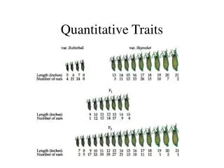
1. Lecture 23: Quantitative Traits III Date: 11/12/02 Single locus backcross regression Single locus backcross likelihood F2 – regression, likelihood, etc

2. Backcross Model m1 is the genotypic value of QQ m2 is the genotypic value of Qq

3. Backcross – t-test

4. Backcross – Linear Regression (BLG) • One may also test the data using a simple linear regression model. • Where yj is the trait value for the jth individual, xjis a dummy variable indicating marker genotype (AA or Aa). • You know that estimates of the coefficients are given by: • We seek the expectation of these coefficients under a genetic model.

5. BLG – Expected Sample Statistics • To find the expected values under the genetic model, we need the expectation of the sample means and variances:

6. BLG – Expected Coefficients • Recalling the coefficient estimators: • Finally, recalling our genetic models:

7. BLG – Hypothesis Testing • We conclude that the expected regression coefficient is: • So, again, rejecting H0: b=0 means • q=0.5 (NO LINKAGE) • a=0 or a=d=0 (NO VARIATION) • k=±1 or a=d (COMPLETE DOMINANCE)

8. Backcross – Likelihood (BL) • One may also set up a likelihood function for backcross progeny. • Trait values are assumed approximately normal (lots of little effects added together). • The distribution of trait values for each marker class are assumed to be a mixture of two normals, one for each possible genotype at the QTL. • The mixing proportions are determined by the recombination fraction.

9. BL – Distributions Class AA Suppose q=0.2 80% QQ 20% Qq m1 mAA m2

10. BL – Distributions Class Aa Qq 80% QQ 20% m1 mAa m2

11. BL – Assumptions • Assume the trait variances for the two QTL genotypes in the backcross are equal. • Assume the traits are normally distributed. • Assume there is no marker / trait interaction, so the distributions remain unchanged in both marker classes (i.e. same variances).

12. BL – Likelihood • The likelihood function for the backcross is then: • where Qj is one of the (unknown) two possible genotypes at the marker locus.

13. BL – Log Likelihood • Take the log of the likelihood to obtain:

14. BL – Null Hypothesis A • One null hypothesis of interest is that the mean genotypic values for the two distributions are not in fact different, so H0: m1 = m2 = m. • In this case, the log likelihood becomes:

15. BL – Null Hypothesis B • Another, perhaps more interesting null hypothesis, is that there is no linkage, so H0: q=0.5 • Under this assumption, the log likelihood becomes

16. BL – Statistical Test • The G statistic that is commonly calculated to test for linkage is: • However, this test is less powerful than the t test introduced earlier.

17. BL – LOD Scores • Again, LOD scores are commonly used for QTL detection. • Where, we interpret, as usual, that a lod score of l means the alternative hypothesis is 10l times as likely as the null hypothesis.

18. BL – Likelihood Maximization • Analytic solutions are difficult to achieve. • Iterative approaches are generally used (EM, NR). • Combinations of methods are also used. For example, the variance is commonly estimated with the pooled variance:

19. BL – Likelihood Maximization • To facilitate calculations even more, a grid of q values with maximization on m1 and m2 can be used. • So suppose you have multiple markers with known map position. Then, evaluate a G statistic or lod score for 3 possible locations of the QTL:

20. BL – Sample Results

21. BL – Caveats • When there is more than one QTL in the same vicinity, the peaks in the LOD score plot may not correspond to QTLs. • Recall that these results are still based on single-locus analysis for which we cannot separate genetic effect from linkage. Thus, there is little good information about QTL location in such a plot, even though it looks like there should be.

22. BL – Comments • Note, that if marker density is high, then there is no need to evaluate at multiple levels of q for each marker. • However, when marker density is low, information is gained when multiple QTL locations are considered. • When q=0 is assumed, the estimates of m1 and m2 are simple means.

23. Single Marker F2 (F2) • There are now three possible genotypes to consider for both the marker and the QTL locus.

24. F2 – Expected Trait Values QQ qq Qq -a a d

25. F2 – Dominant Marker • Similar tables can be derived for the case of a dominant marker. • In general, the procedure is as follows: • Derive the QTL genotype probabilities conditional on the marker phenotype. • Using the conditional probabilities, derive the expected trait value for each marker phenotype class.

26. F2 – Regression (F2R) • The regression model is • where yj is the trait value of the jth individual in the population • where x1j is the dummy variable for marker additive effect taking on value 1 for AA, 0 for Aa, and –1 for aa. • where x2j is the dummy variable for marker dominance effect taking on value 1 for AA and –1 for Aa and 1 for aa.

27. F2R – Matrix Notation

28. F2R – Expected Coefficients • The coefficient estimates have expectation:

29. F2R – F Statistics • The F statistic is the ratio between the residual mean squares for the reduced model and the full model. • The full model has residual mean square:

30. F2R – Reduced Models • Reduced models of interest are: • And the F statistics are:

31. F2R – Dominant Marker • If the marker locus segregates as a dominant trait, then: • Thus, significant regression coefficient tests for a confounded additive effect, dominance effect, and linkage.

32. F2 – Likelihood Approach (F2L) • Assume trait variances for the three QTL genotypes are equal. • For each marker class, the trait value is a mixture of three normal distributions with different means, equal variances, and expected proportions based on degree of linkage. • The expected proportions are given in slide #23.

33. F2L – Log Likelihood • The likelihood then becomes a sum over three normals:

34. F2L – Null Hypothesis A • If the null hypothesis is H0: a = 0

35. F2L – Null Hypothesis B • Suppose instead that the null hypothesis is H0: d = 0

36. F2L – Null Hypothesis C • Suppose instead that the null hypothesis is H0: a = 0, d = 0

37. F2L – Null Hypothesis D • When the null hypothesis is H0: q= 0.5

38. F2L – Statistical Test • The G statistic

39. F2L – Maximization • Iterative methods are required to find the maximum likelihood estimates. • Other approaches have been suggested, such as combining moment estimation with maximum likelihood approach. The resulting system of equations to solve for the estimators is given on the next slide.

40. F2L – Finding MLEs

41. F2L – Dominant Marker Model • Modify the likelihood equations with QTL genotypes probabilities conditional on the marker genotype for a dominant marker. • Modify the expected trait values for each marker genotype. • Done.