
Spline Interpolation: Cubic and Higher-Degree Polynomials
E N D
Presentation Transcript
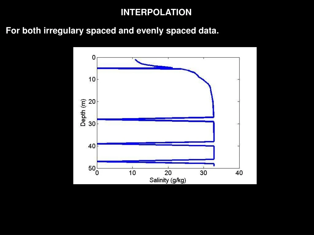
INTERPOLATION For both irregulary spaced and evenly spaced data.
Linear Interpolation y x = a x x = b x
Spline interpolation – we approximate the interpolation function y(x) over the interval [a, b] by dividing the interval into subregions. The function should be continuous at the joints. Define spline function y(x) of degree N with values @ joints: b a data need to be in ascending (or descending order); if not, it should be rearranged Spline function y(x) has two properties: a) In each interval ui-1xui(i = 1,…, m), the function y(x) is a polynomial of degree < N. b) At each interior joint, y(x) and its first N-1 derivatives are continuous.
The most common spline function is the cubic spline N = 3 Example. Consider a data series with elements (xi, yi), i =1, …, N The first two derivatives y’(x) and y’’(x) of the interpolation function can be defined for all xi The third derivative y’’’(x) is a constant for all x At the segment junctions: Continuity of the spline function Continuity of the slope Continuity of the curvature
Since y’’’(x) is a constant, y’’(x) must be linear, so that Integrating twice, getting integration constants from a) continuity of the function and b) of the slope:
Cubic Spline Fifth degree polynomial Sixth degree polynomial Eighth degree polynomial = cubic spline for this example
clear all close all x=[3 4.5 7 9]; y=[2.5 1 2.5 .5]; plot(x,y,'o','MarkerFaceColor','red','MarkerSize',10) axis([2 10 0 3]) ; set(gca,'FontSize',18) x1=[3:.25:9]; y1=interp1(x,y,x1); hold on plot(x1,y1,'b','LineWidth',3) y2=interp1(x,y,x1,'spline'); plot(x1,y2,'r','LineWidth',4) %Shape-preserving piecewise cubic interpolation. %The interpolated value at a query point is based on a shape-preserving %piecewise cubic interpolation of the values at neighboring grid points. y3=interp1(x,y,x1,'pchip'); plot(x1,y3,'k','LineWidth',2)