Download

1 / 41
410 likes | 453 Views
Delve into the intricate world of temporal niche partitioning in vertebrates, focusing on how different species adapt their activity times to optimize resource utilization. Discover the seasonal variations, diurnal differences, and predator behaviors that shape these temporal niches.

E N D
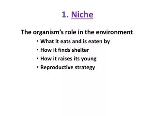
Temporal Niche • Time as a resource axis • Consider activity times of vertebrates • Owls vs. hawks
Temporal Niche Time as a resource axis Seasonal differences in flowering times (lowering competition for pollinators)
Temporal Partitioning • Animals can move • But animals must constantly forage • Plants must cope with constant competition from neighbors • Most plants can persist through resource droughts
Temporal Niche A traditional model of competition (exploitive) does not really view time as an independent axis
Temporal Niche • There are two ways in which time may be partitioned: • 1) seasonal differences may allow predators to coexist by exploiting different prey assemblages • 2) diel differences may allow predators to partition a rapidly renewing resources
Temporal Niche • Schoener (1974) reviewed the early literature and determined animals often segregate food and habitat dimensions but rarely segregate along temporal niche axis • Predators utilized diel partitioning more than other trophic groups • So, what has gone on…
Temporal Niche • You could treat time as any other niche axis (and reshuffle observed activity data) • For example, Pianka looked at seasonal activity (or daily activity) • Results, time was not important (food overlap study showed significant differences)
Temporal Niche • Although RA1-RA4 are all valid null models for looking many overlap studies (e.g. diet or microhabitat) they may not be appropriate for temporal niche studies • Most species show strong modalities with peak activity at certain times (again daily or seasonal) or multiple times • RA1-RA4 are going to ‘destroy’ the curves
Temporal Niche • A more appropriate null model may be to retain the shape of the activity curve and randomize the placement of its peak
Temporal Niche One important assumption of temporal activity patterns is that animals that feed at different times must have different diets • For example, nocturnal and diurnal predators should differ in their diets and therefore face less competition from each other than with species with an identical activity level
Temporal Niche • One appropriate null model would be the dietary overlap between species with similar activity patterns (matched) is no different than for a random ‘mixed’ pair (one diurnal and one nocturnal species) • Would your alternative hypothesis be temporal aggregation or segregation? • Why and what is the mechanism?
Temporal Niche • Jaksic (1982) tested these hypotheses for dietary overlaps of diurnal falconiform and nocturanal strigiform raptors. • Results (using standard nonparametric statistics) indicated there were no significant differences in dietary overlap of mixed versus matched species pair • Thus no exploitative competition demonstrated (what about interference?)
Temporal Niche • However, standard statistics may not be suitable for testing the mixed-matched dietary overlap hypothesis (think independence of Sp A,B and C) • Also, nearest-neighbor statistic is biased; consider large sample vs. small A & B, B & C, C& A
Temporal Niche • Calculating a new overlap score for each random pair would yield a null model (Pimm 1983) (e.g. consider a group noctural and diurnal predators) • We would expect matched pairs (lower) and mixed (higher) should differ from random. Furthermore, nearest neighbor should be a smaller distance than random
Temporal Niche • Huey and Pianka (1983) examined dietary differences between nocturnal and diurnal predators in assemblages of lizards, raptors and water snakes • For both African and Australian lizards, significantly more first- and second-nearest neighbors in dietary similarity were synchronous than were asynchronous in the activity times
Temporal Niche • Similarly, more synchronous pairs of species tended to overlap in diet more often than predicted, and synchronous pairs less often than predicted (opposite of the predictions of the mixed-matched dietary hypothesis, suggesting that lizard food resources are not being partitioned by species that are active at different times of the day)
Temporal Niche • Fig 5.2
Temporal Niche • For raptors, were not different than their null model • For water snakes, dietary overlap of synchronous species were higher than expected • Consequently, the degree of synchrony in activity periods is not a reliable indicator of dietary overlap
Phenological Overlap There are alternative hypotheses for the evolution of nocturnal and diurnal segragation … Predator avoidance Alleviation of interference competition Physiological constraints
Temporal Niche • Seasonal overlap may be more plausible than daily • Hypothesized that within functional feeding guilds of stream insects, competition for food will result in temporal segregation (apparent sequential peak production of six species in an Appalachian stream)
Phenological Overlap • Robertson (1895) first proposed that pollen transfer by animals was a potentially limiting resource that could lead to staggered phenologies of flowering plants • However, other hypotheses also exist…
Phenological Overlap • 1) pollinator preference in which one species is a winner (and others lose) • 2) interspecific pollen transfer (resulting in lower reproductive success of some sort) • 3) formation of maladaptive hybrids (again lowering fitness) • Mechanism (1) suggests competition for competitors, (2) does not; all 3 suggest increases in abundance of one plant species and its’ pollinators can be negative
Phenological Overlap However, there is a specific case when some plants can be benefited from the presence of others plants… when?
Phenological Overlap • Segregation of flowering times will reduce overlap in shared pollinators. However, is the converse true? • High overlap in flowering times need not imply strong competition for pollinators • Thompson (1982) found overlaps in flowering times of subalpine meadow plants were unrelated to relative visitation rates by pollinators
Phenological Overlap • Despite the attention phenological studies have received, there had been little statistical investigation Fig 5.3
Phenological Overlap • Poole and Rathcke (1979) summarized overlap as a single index (the sample variance of the distance between adjacent flowering peaks; similar to body size spacing). • The distance from first to last flowering represents the range (0 to 1) if competition has lead to regular spacing of the other species
Phenological Overlap • If competition has led to regular spacing of peak flowering times, the observed (population) variance in the position of lowering peaks should be significantly smaller than expected by chance
Phenological Overlap • The ratio of observed to expected variance (P/E(P) is an idex that correspnds to flowering peaks that aggregated (if (P/E(P) > 1), random (P/E(P) =1, or staggered (P/E(P) <1) with the growing season. • **This metric is the same for determining the spatial structure of distributions
Phenological Overlap • Stiles claimed lowering peaks exhibited an orderly, staggered sequence
Phenological Overlap Later found to be slightly staggered
Phenological Overlap • Remember, this metric does not measure overlap in flowering times, but regularity in the spacing of peak flowering times • Cole (1981) proposed a different metric, which represents the flowering period as a line segment rather than representing the flowering peak as a single point, then calculating overlap of the line segment
Phenological Overlap • The null hypothesis is simply that the flowering period of each species occurs randomly and independently within the growing season • Statistical analysis is problematic (non-independence of overlaps) • There have been many other iterations of various metrics
Phenological Overlap • Ashton et al. (1988) pointed out that since the boundaries of flowering times are bound by observed data and randomizations all occur within those boundaries, they are biased towards ‘low-overlap’ patterns • Note: most simulations have detected random or aggregated patterns
Phenological Overlap • Their solution was to also use peaks, but expand the boundaries of the ‘season’ to possibly include all dates
Nonequilibrium Analyses • The preceding analyses all make the implicit assumption that flowering times or activity periods of species have reached an ecological or evolutionary equilibrium • There are a number of different mechanisms that may structure a community
NonequilibriumAnalyses • If communities are in equilibrium, the phenological pattern of temporal overlap from one year to the next would be consistent (as well as the opposite pattern) • If resources fluctuate, then competitive effects may be only seen during ‘resource crunches’
Nonequilibrium Analyses • What would constitute a valid null model for assessing equilibrium? • One approach would be to assess if co-occurring species exhibit compensatory fluctuations in abundance, activity, or phenology • If a community is in equilibrium, then relative changes in abundance should be mirrored (inversely) by other species • Conversely, positive fluctuations may occur if species are tracking shared resources
Nonequilibrium Analyses • What would the data look like? • Jan March May July Sept Nov • Sp A 5 10 15 10 4 4 • Sp B 6 12 14 12 6 6 • Sp C 5 10 15 10 4 4 • Patterns of covariance in this matrix can be quantified by comparing the sum of the individual species variances to the variance of their sums
NonequilibriumAnalyses Specifically, the ratio of variance of their sums to the variance of the individual species (V) This ratio describes whether species are fluctuating independently (V=1), concordantly (V>1), or compensatorily (V<1) One important variant, the product of the variance ratio and the number of censuses (VT) can be used as a significance test
Summary There are good tests to compare diets of synchronous and asynchronous predators (Pimm’s Monte Carlo simulation) Flowering peaks (Poole and Rathcke, although maybe better (chap 6)) Flowering intervals (Ashton et al) Compensatory fluctuations of abundance or activity (Schulter’s variance ratio)