Download
1 / 27
280 likes | 403 Views
This chapter delves into key aspects of variable transformations in regression analysis, focusing on how rescaling affects coefficients and statistical metrics while preserving overall results. It provides practical examples using datasets like 4th Graders' Foot Measurements and TV Advertising Budgets. Learn about beta coefficients, z-scores, the impact of logarithmic transformations, and quadratic effects on modeling variables. Emphasis is placed on interpreting regression outputs, R-squared values, and adjusted R-squared, offering insights into better predictive modeling in time series analysis.

E N D
Units Conversions When variables are rescaled (units are changed), the coefficients, standard errors, confidence intervals, t statistics, and F statistics change in ways that preserve all measured effects and testing outcomes.
Beta Coefficients A z-score is: In a data set, the data for each regression variable (independent and dependent) are converted to z-scores. Then, the regression is conducted.
Beta Coefficients – Example Use the data set 4th Graders Feet Regress foot length on foot width The regression equation is Foot Length = 7.82 + 1.66 Foot Width Predictor Coef SE CoefT P Constant 7.817 2.938 2.66 0.011 Foot Width 1.6576 0.3262 5.08 0.000 S = 1.02477 R-Sq = 41.1% R-Sq(adj) = 39.5%
Beta Coefficients – Example Use the data set 4th Graders Feet Regress z-score of foot length on z-score of foot width The regression equation is zFoot Length = - 0.000 + 0.641 zFoot Width Predictor CoefSE CoefT P Constant -0.0000 0.1245 -0.00 1.000 zFoot Width 0.6411 0.1262 5.08 0.000 S = 0.777763 R-Sq = 41.1% R-Sq(adj) = 39.5%
Using the Log of a Variable Taking the log usually narrows the range of the variable – This can result in estimates that are less sensitive to outliers
Using the Log of a Variable When a variable is a positive $ amount, the log is usually taken When a variable has large integer values, the log is usually taken: population, total # employees, school enrollment, etc…
Using the Log of a Variable Variables that are measured in years such as education, experience, age, etc… are usually left in original form
Using the Log of a Variable Proportions or percentages are usually left in original form because the coefficients are easier to interpret – percentage point change interpretation.
Modeling a Quadratic Effect Consider the quadratic effect dataset Want to predict Millions of retained impressions per week Predictor is TV advertising budget, 1983 ($ millions) Model is:
Consider the quadratic effect dataset Want to predict Millions of retained impressions per week Predictor is TV advertising budget, 1983 ($ millions) The regression equation is MIL = 22.2 + 0.363 SPEND Predictor Coef SE CoefT P Constant 22.163 7.089 3.13 0.006 SPEND 0.36317 0.09712 3.74 0.001 S = 23.5015 R-Sq = 42.4% R-Sq(adj) = 39.4%
Modeling a Quadratic Effect Consider the quadratic effect dataset Want to predict Millions of retained impressions per week Predictor is TV advertising budget, 1983 ($ millions) Add the quadratic effect to the model Model is:
Model is: The regression equation is MIL = 7.06 + 1.08 SPEND - 0.00399 SPEND SQUARED Predictor CoefSE CoefT P Constant 7.059 9.986 0.71 0.489 SPEND 1.0847 0.3699 2.93 0.009 SPEND SQUARED -0.003990 0.001984 -2.01 0.060 S = 21.8185 R-Sq = 53.0% R-Sq(adj) = 47.7%
Modeling a Quadratic Effect The interpretation of the quadratic term, a, depends on whether the linear term, b, is positive or negative.
The graph above and on the left shows an equation with a positive linear term to set the frame of reference. When the quadratic term is also positive, then the net effect is a greater than linear increase (see the middle graph). The interesting case is when the quadratic term is negative (the right graph). In this case, the linear and quadratic term compete with one another. The increase is less than linear because the quadratic term is exerting a downward force on the equation. Eventually, the trend will level off and head downward. In some situations, the place where the equation levels off is beyond the maximum of the data.
Quadratic Effect Example Consider the dataset MILEAGE (on my website) Create a model to predict MPG
More on R2 R2 does not indicate whether The independent variables are a true cause of the changes in the dependent variable omitted-variable bias exists the correct regression was used the most appropriate set of independent variables has been chosen there is collinearity present in the data on the explanatory variables the model might be improved by using transformed versions of the existing set of independent variables
More on R2 But, R2 has an easy interpretation: The percent of variability present in the independent variable explained by the regression.
Adjusted R2 Modification of R2 that adjusts for the number of explanatory terms in the model. Adjusted R2increases only if the new term added to the model improves the model sufficiently This implies adjusted R2 can rise or fall after the addition of a new term to the model. Definition: Where n is sample size and p is total number of predictors in the model
Adjusted R2 – Example Use MILEAGE data set Regress MPG on HP, WT, SP What is the R2 and the adjusted R2 Now, regress MPG on HP, WT, SP, and VOL What is the R2 and the adjusted R2
Prediction Intervals Use MILEAGE data set Regress MPG on HP We want to create a prediction of MPG at a HP of 200 Minitab gives: New Obs Fit SE Fit 95% CI 95% PI 1 22.261 1.210 (19.853, 24.670) (9.741, 34.782)
Prediction Intervals Difference between the 95% CI and the 95% PI Confidence interval of the prediction: Represents a range that the mean response is likely to fall given specified settings of the predictors. Prediction Interval: Represents a range that a single new observation is likely to fall given specified settings of the predictors. New Obs Fit SE Fit 95% CI 95% PI 1 22.261 1.210 (19.853, 24.670) (9.741, 34.782)
Prediction Intervals Model has best predictive properties – narrowest interval – at the means of the predictors. Predict MPG from HP at the mean of HP