Download
1 / 58
580 likes | 618 Views
Learn about the various types of space-filling curves including the Hilbert, Peano, Sierpinski, and Lebesgue curves, and discover their applications. Presented by Levi Valgaerts at JASS 2005 in Saint Petersburg.

E N D
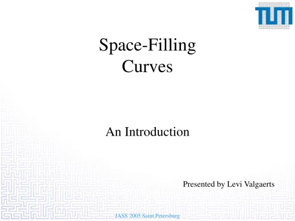
Space-FillingCurves An Introduction Presented by Levi Valgaerts JASS 2005 Saint Petersburg
Contents • Introductory section • Types of space-filling curves • The Hilbert space-filling curve • The Peano space-filling curve • The Sierpinski space-filling curve • The Lebesgue space-filling curve • Application of space-filling curves JASS 2005 Saint Petersburg
Contents • Introductory section • Types of space-filling curves • The Hilbert space-filling curve • The Peano space-filling curve • The Sierpinski space-filling curve • The Lebesgue space-filling curve • Application of space-filling curves JASS 2005 Saint Petersburg
Basic concepts from set theory: surjective, injective, bijective mapping • Surjective map from A onto B:withthe image of A under the function f JASS 2005 Saint Petersburg
Basic concepts from set theory: surjective, injective, bijective mapping • Injective map from A into B: • Bijective map from A onto B:f is injective and surjective JASS 2005 Saint Petersburg
Basic notations • Subsets of : , • Binary notation:Ternary notation:Quaternary notation: JASS 2005 Saint Petersburg
Basic notations (remarks) • Periods • Finite binariese.g. because JASS 2005 Saint Petersburg
Curve definition If is continuous, then is called a curve. Without loss of generality we can assume the domain to be I, f(0) and f(1) are the beginning and endpoint. Notation: Parameter representation with component functions: JASS 2005 Saint Petersburg
Space-filling curve (SFC) definition Curves that pass through every point of an n-dimensional region with positive area (for n=2) or volume (for n=3), such as the unit square Ω in or the unit cube in , are called space-filling curves. Two main characteristics: • continuous • surjective It can be shown that if f generates a space-filling curve, then it can not be bijective. JASS 2005 Saint Petersburg
Contents • Introductory section • Types of space-filling curves • The Hilbert space-filling curve • The Peano space-filling curve • The Sierpinski space-filling curve • The Lebesgue space-filling curve • Application of space-filling curves JASS 2005 Saint Petersburg
Contents • Introductory section • Types of space-filling curves • The Hilbert space-filling curve • The Peano space-filling curve • The Sierpinski space-filling curve • The Lebesgue space-filling curve • Application of space-filling curves JASS 2005 Saint Petersburg
The Hilbert curve: geometric generation • If I can be mapped continuously on Ω, then after partitioning I into four congruent subintervals and Ω into four congruent subsquares, each subinterval can be mapped continuously onto one of the subsquares. This partitioning can be carried out ad infinitum. • The subsquares must be arranged such that adjacent subintervals are mapped onto adjacent subsquares. • Inclusion relationship: if an interval corresponds to a square, then its subintervals must correspond to the subsquares of that square. • This process defines a mapping , called the Hilbert space-filling curve. JASS 2005 Saint Petersburg
1/4 2/4 3/4 4/4 0 1 1/16 2/16 3/16 4/16 16/16 1,1 1,1 2 3 1st iteration 3rd iteration 2nd iteration 4 3 1 4 1 2 16 0,0 0,0 The Hilbert curve: geometric generation JASS 2005 Saint Petersburg
The Hilbert curve: geometric generation 6th iteration JASS 2005 Saint Petersburg
The Hilbert curve: geometric generation The mapping is surjective: with every sequence of nested closed squares corresponds a sequence of nested closed intervals that define a unique . The mapping is continuous: in the nth iteration I is partitioned in subintervals, thus The mapping is nowhere differentiable. JASS 2005 Saint Petersburg
The Hilbert curve: a complex representation [Sagan] • Establish a formula to calculate the exact coordinates of an image point if • Use complex representation , and affine transforma-tions to wich Ω will be subjected recursively. • Give an orientation to each subsquare such that the exit point of a subsquare coincides with the entry point of the next subsquare. JASS 2005 Saint Petersburg
0 1 1 0 1 0 0th iteration 1st iteration 2nd iteration The Hilbert curve: a complex representation JASS 2005 Saint Petersburg
The Hilbert curve: a complex representation The four basic transformations (2 dimensional case): JASS 2005 Saint Petersburg
The Hilbert curve: a complex representation • Represent as • , , ad infinitum: • For finite quaternaries (edges of subintervals in nth iteration): JASS 2005 Saint Petersburg
The Hilbert curve: a complex representation • continued... • Taking into account some properties of : JASS 2005 Saint Petersburg
(0,0) The Hilbert curve: a complex representation • Further simplifications of the formula are possible... • An example: JASS 2005 Saint Petersburg
Approximating polygons for the Hilbert curve The polygonal line that runs through the points is called the nth approximating polygon or a discrete space filling curve. Parametrization: converges uniformly to the Hilbert curve JASS 2005 Saint Petersburg
The Hilbert curve: representation through grammars • Make use of four distinct templates to generate the discrete Hilbert curve: H,A,B and C. • These templates will be translated to a first iteration of the curve according to a fixed scheme. JASS 2005 Saint Petersburg
The Hilbert curve: representation through grammars • The resulting rules and transitions can be used to implement the recursive construction of the discrete Hilbert curve. JASS 2005 Saint Petersburg
3 dimensional SFCs JASS 2005 Saint Petersburg
Contents • Introductory section • Types of space-filling curves • The Hilbert space-filling curve • The Peano space-filling curve • The Sierpinski space-filling curve • The Lebesgue space-filling curve • Application of space-filling curves JASS 2005 Saint Petersburg
Contents • Introductory section • Types of space-filling curves • The Hilbert space-filling curve • The Peano space-filling curve • The Sierpinski space-filling curve • The Lebesgue space-filling curve • Application of space-filling curves JASS 2005 Saint Petersburg
The Peano curve: definition • with is surjective and continuous on I, and represents a SFC. • More interesting: geometric generation according to Hilbert JASS 2005 Saint Petersburg
1 3 4 9 2 5 8 1 6 7 0 1 The Peano curve: geometric generation From the defining formula we can derive: • ... JASS 2005 Saint Petersburg
1st iteration 2nd iteration 3rd iteration The Peano curve: geometric generation JASS 2005 Saint Petersburg
The Peano curve: a complex representation • Define orientation of the subsquares: • Define similarity transforms:with JASS 2005 Saint Petersburg
The Peano curve: a complex representation • Use ternary representation of : • Continue as with Hilbert´s curve... we get the same result as in Peano´s definition JASS 2005 Saint Petersburg
Approximating polygons for the Peano curve JASS 2005 Saint Petersburg
The Peano curve: representation through grammars JASS 2005 Saint Petersburg
Contents • Introductory section • Types of space-filling curves • The Hilbert space-filling curve • The Peano space-filling curve • The Sierpinski space-filling curve • The Lebesgue space-filling curve • Application of space-filling curves JASS 2005 Saint Petersburg
Contents • Introductory section • Types of space-filling curves • The Hilbert space-filling curve • The Peano space-filling curve • The Sierpinski space-filling curve • The Lebesgue space-filling curve • Application of space-filling curves JASS 2005 Saint Petersburg
The Sierpinski curve: generation Originaly defined as a map from I onto , but it can be considered as a map from I onto a right isosceles triangle . JASS 2005 Saint Petersburg
t n=2 n=1 n=0 The Sierpinski curve: generation • Partition I into congruent subintervals and into congruent subtriangles. • In deriving an algabraic representation it is easier to divide I into subintervals, thus using quaternaries: JASS 2005 Saint Petersburg
The Sierpinski curve: generation with similarity transforms: JASS 2005 Saint Petersburg
The Sierpinski curve: generation • Taking into account some properties of : JASS 2005 Saint Petersburg
t n=3 n=2 n=1 n=0 The Sierpinski curve: approximating polygons JASS 2005 Saint Petersburg
Contents • Introductory section • Types of space-filling curves • The Hilbert space-filling curve • The Peano space-filling curve • The Sierpinski space-filling curve • The Lebesgue space-filling curve • Application of space-filling curves JASS 2005 Saint Petersburg
Contents • Introductory section • Types of space-filling curves • The Hilbert space-filling curve • The Peano space-filling curve • The Sierpinski space-filling curve • The Lebesgue space-filling curve • Application of space-filling curves JASS 2005 Saint Petersburg
The Lebesgue curve: introduction Introduction of a remarkable subset of I, the Cantor Set ,of wich all elements can be represented by may be constructed by recursively removing the middle third of every closed subinterval beginning with I. The numbers that are generated in this proces do not contain a 1 in their ternary representation. JASS 2005 Saint Petersburg
The Lebesgue curve: introduction • ... JASS 2005 Saint Petersburg
The Lebesgue curve: definition We define the continuous and surjective mapping and extend f continuously into I by linear interpolation in every interval that is removed in the generation of : with removed in the nth iteration step. Further we say on . Than defines the Lebesgue space-filling curve. JASS 2005 Saint Petersburg
2nd iteration 4th iteration 1st iteration The Lebesgue curve: generation and approxima-ting polygons JASS 2005 Saint Petersburg
Contents • Introductory section • Types of space-filling curves • The Hilbert space-filling curve • The Peano space-filling curve • The Sierpinski space-filling curve • The Lebesgue space-filling curve • Application of space-filling curves JASS 2005 Saint Petersburg
Contents • Introductory section • Types of space-filling curves • The Hilbert space-filling curve • The Peano space-filling curve • The Sierpinski space-filling curve • The Lebesgue space-filling curve • Application of space-filling curves JASS 2005 Saint Petersburg
Application of space-filling curves 2 dimensional SFCs give a recipe for going through a set of 2 dimensional data that are arranged on a grid: • going through pixels that make up an image being scanned • matrix operations in linear algebra • going through / representing a 2D computational grid • ... Favorable property: better exploitation of the 2D locality due to the recursive nature / self-similarity. JASS 2005 Saint Petersburg