Download
1 / 32
330 likes | 363 Views
Learn about space-filling curves like Hilbert's and Peano's and their usage in numerical simulations with hierarchical basis systems for FEM analysis efficiency.

E N D
Agenda • Motivation • Space filling curves • Definition • Hilbert’s space filling curve • Peano’s space filling curve • Usage in numerical simulations • Hierarchical basis and generating systems • Standard nodal basis for FEM-analysis • Hierarchical basis • Generating systems
1. Motivation Time needed for simulating phenomena depends on both performing the corresponding calculation steps and transferring data to and from the processor(s). • The latter can be optimised by arranging the data in an effective way to avoid cache misses and support optimisation techniques (e.g. pre-fetching). Standard organization in matrices / arrays leads to bad cache behaviour. Space-Filling Curves • Use (basis) functions for FEM-analysis with which LSE solvers show faster convergence • Hierarchical Basis • Generating System (for higher dimensional problems)
2.a Definition of Space-Filling Curves We can construct a mapping from a 1-D interval to a n-D interval where n is finite, i.e. we can construct mappings as follow: If the curve of this mapping passes through every point of the target space we call this a “Space-Filling Curve”. We are interested in a continuous mapping. This cannot be bijective, it’s only surjective.
Remark:When moving a certain distance on the unit interval we can easily estimate the possible position in the target space (~ radius). 2.a Geometric Interpretation 0 1/9 2/9 1 First we partition the interval I into n subintervals and the square into n sub squares. Now one can easily establish a continuous mapping between these areas. This idea holds for any finite-dimensional target space. It’s not necessary to partition into equally sized areas! 1,1 0,0 1/3,0 1,0
1/4 2/4 3/4 4/4 0 1 1/16 2/16 3/16 4/16 16/16 1,1 1,1 2 3 4 3 1 4 1 2 16 0,0 0,0 2.b Hilbert’s Space-Filling Curve The German mathematician David Hilbert (1862-1943) was the first one to give the so far only algebraically described space-filling curves a geometric interpretation. In the 2 dimensional case he splat I into four subintervals and into four sub squares. This splitting is recursively repeated for the emerging subspaces, leading to the below shown curve. An important fact is the so called full inclusion: whenever we further split a subinterval, the mapping to the corresponding finer sub squares stays in the former interval. Repeating the partitioning symmetrically (for all subspaces) again and again leads to 22n subintervals / sub squares in case of a 2-dimensional target space. (n: # of partitioning steps)
0 1 1/9 2/9 3/9 4/9 5/9 6/9 7/9 8/9 1,1 3 4 9 7 8 9 2 5 8 6 5 4 1 6 7 1 2 3 0,0 2.c Peano’s Space-Filling Curve The Italian mathematician Giuseppe Peano (1858-1932) was the first one who constructed (only algebraically) a space filling curve in 1890. According to him we split the starting domain into 3m sub areas. The Peano curve goes always from 0 to 1 in all dimensions. The way we run through the target space is up to us.Two different ways are marked with blue / red numbers. Only the first and the last subspaces are mapped in a fixed way. Recursive partitioning leads to finer curves (compare with Hilbert’s curve). Symmetrical partitioning leads to 3mn sub areas. m: # dim() n: # of partitioning steps
We begin with the unit cube. The Peano curve begins in (0,0,0) and ends in (1,1,1). 1/3,1,1 1,1,1 1,1,1 0,0,0 0,0,0 2/3,0,0 2.c Peano curve in 3-D Now we begin to split this cube into finer sub cubes. We can select the dimension we want to begin with.
Now the emerging sub spaces are split in one on the two remaining dimensions. 1/3,1,1 1/3,1,1 1,1,1 1,1,1 1,1/3,1 1,1/3,1 2/3,0,2/3 1,1/3,1/3 0,0,0 0,0,0 2/3,0,0 2/3,0,0 2.c Peano curve in 3-D (continued) After splitting the sub spaces in the last dimension we end up with 27 equally sized cubes (symmetrical case, here: 7 cuboids.)
2.d Usage in numerical simulations 1,1 • So far we’ve only spoken about the generation of space filling curves. But how can this be of advantage for the data transfer in numerical simulations? • To answer this question let’s have a short look at a simple grid. Within a square we need the values at the corner points of that square. When we go through this square following e.g. Peano’s space filling curve we can build up inner lines of data points, which are processed in a forward or backward order. • This scheme corresponds to a stack, on which we can only access the very most upper element (forward: writing to stack, backward: reading from stack). In our example we would need 2 stacks (blue and red). 0,0
In the first square we need the data points 1,2,5,6. Stacks after processing the first cell: stack 1: stack 2: In the second square the points 2,3,6,7 are needed. Stacks after processing the second cell: stack 1: stack 2: 5 6 1 2 1 5 12 1 6 2 11 2 7 3 3 10 Now we jump to the 5th square, points 6,7,10,11 have to be accessed. Stacks after processing the fifth cell: stack 1: stack 2: 5 6 4 8 2.d Example for stack usage Let’s examine what’s happening in the squares. 13 14 15 16 9 10 11 12 5 6 7 8 1 2 3 4
1 17 18 19 16 6 5 15 14 13 10 11 12 9 8 7 2 3 4 2.d Usage with adaptable grids To guarantee the usage of this idea for complex computations it has to hold for adaptable grids, too. We start with the first square on the coarsest grid and recursively refine where needed (remark: full inclusion). This leads to a top-down approach where we first process the cells on the deeper level before finishing the cells on the coarser level. top-down depth-first (When entering cell 6 first we first process cell 6, then cells 7 to 15 are finished and afterwards we return to the coarse level and proceed with cell 16.)
27 1 30 16 26 2 29 17 25 3 18 28 6 31 22 15 23 5 32 14 33 13 24 4 36 21 7 10 35 11 20 8 34 9 12 19 2.d Stacks for adaptable grids Points 1 and 2 are used to calculate cells on both coarse and fine level. When working with hierarchical grid we only have the points 1a and 2a. If we would only use two stacks we would have to store the points 3 and 4 to the same stack as points 1a and 2a. When finishing fine cell 9 (fine level) point 4 would lie on top of the stack containing point 2a, cell 3 (coarse level) couldn’t access point 2a. We handle this problem by introducing two new stacks. We use 2 point stacks (0D) and 2 line stacks (1D). When working with a generating system we have different point values on all levels (points 1a,1b and 2a, 2b). 7 8 9 6 5 4 2b 1a 2a 1b 3 1 2 3 4
0,1 21 1,1 0,0,1 201 1,0,1 02 22 12 002 202 102 0,0 20 1,0 0,0,0 200 1,0,0 2.d Stacks in adaptable grids & generating systems As already mentioned, with generating systems we have point values on different levels. To deal with these problems the so far used number of stacks is insufficient. One can show that the number of stacks can be calculated the way shown below. We numerate the points according to their value in the Cartesian coordinate system. The connecting lines e.g. 02 are numerated the following way (element-wise): • if the corresponding point coordinates are equal: take their value • else write a 2 This leads to the following formula for the # of stacks: 3dim dim = 2 9 stacks (4 point stacks, 4 line stacks, 1 plane stacks = in/output) dim = 3 27 stacks (8 point stacks, 12 line stacks, 6 plane stacks, 1 volume stack = in/output)
2.d Conclusion • Peano-curves allow efficient stack usage for n-dimensional problems. (Hilbert-curves show this advantage only for the 2-dimensional case, as the higher dimensional curves don’t show exploitable behaviour.) • The number of needed stacks is independent of the problem size. computation speed-up due to efficient cache usage (CPU pre-fetching unit can efficiently load the needed data when organised in an easy way.) • The only drawback is the recursive splitting into 3n subintervals when using Peano curves which lead to more points, but we gain more than we loose here.
ith hut-function 0 1 xi-1 xi xi+1 A set of linear independent hut-functions forms a basis of the solution space. (boundaries not treated) 0 1 3.a Standard nodal basis for FEM-analysis FEM – analysis uses a set of independent piece-wise linear functions to describe the solution. We can write the function u(x) as follows: ui: function value at position I i: hut-function which has the value one at position i, zero at the neighbouring positions (i-1, i+1) and is linear between
3.a Resulting LSE (Linear System of Equations) We now have a short look on the one-dimensional Poisson equation using the standard discretization approach. The problem condition depends on the ration max/ min. max goes towards the row sum (= 2) and min tends towards zero, therefore the resulting condition is rather poor. This causes slow convergence.
3.a Drawbacks of standard approach • Slow convergence rate as already shown due to bad eigenvalues. Moreover the condition depends on the problem size! • When we have to examine a certain area in more detail, i.e. when we need locally a higher resolution we cannot reuse the already performed work. We have to calculate new hut-functions. Use hierarchical basis to compensate these two effects.
A possibility to deal with the mentioned drawbacks is to use a hierarchical basis. Unlike with the standard approach we now use all the hut-functions on the coarser levels when refining. On finer levels hut-functions are only created at points which don’t define functions on higher levels. These hut-functions still build up a basis. One can uniquely describe the function u(x) by summing up the different hut-functions on the different levels. standard basis hierarchical basis 3.b Hierarchical Basis
coefficients: ¾ , 1 , ¾ coefficients: ¼ , 1 , ¼ 3.b Interpretation of hierarchical basis • The picture below shows a simple interpolation of a parabola using standard basis (left side) and hierarchical basis (right side). • The coefficients needed for the normal approach are the function values at the corresponding positions. (This is also the reason why one cannot locally refine and reuse older values.) • For the hierarchical basis only the first coefficient equals the corresponding function value (= 1 in below example). The coefficients for the finer levels just describe the difference between the real function value and the one described by all previous hut-functions. This supports reuse when locally refining.
3.b Representation in hierarchical basis Let’s remember the representation of the function u(x) using the nodal basis: The same function u(x) can be represented using a hierarchical basis: Both representations describe the same function. We can define a mapping transforming the normal representation into the hierarchical one:
hierarchical difference (coarse – fine level) coefficient for hierarchical basis v2k+1 u2k+1 u2k 3.b Transformation into hierarchical basis When transforming the coefficients of the standard description into the hierarchical basis we use the following formula: So we can find the entries (-1/2, 1, -1/2) in each row of the transformation matrix H. (We have to use this formula recursively to calculate the coefficients on all levels.) u2k+2
v4 v2 v5 v1 v6 v3 v7 u1 u2 u7 0 1 0 1 3.b Transformation into hierarchical basis (cont.) Let’s examine as example the parabola defined by the points (0,0), (1,1) and (2,0). We are using 7 equally distributed inner points. transformation matrix H coefficients for standard basis(u1,…,u7)’ coefficients for hierarchical basis(v1,…,v7)’
3.b Usage in numerical schemes We want to solve more effectively . To do so we replace the standard representation of u by its hierarchical one. When we now multiply the equation from the left by T’ we’ll end up with a new equation for v(x) (this will be a very nice one). The transformation into u(x) is then easily performed.
v4 v2 v5 v1 v6 v3 v7 u1 u2 u7 0 1 0 1 3.b Transforming v(x) into u(x) Again we consider the transformation for our parabola example. transformation matrix T coefficients for standard basis(u1,…,u7)’ coefficients for hierarchical basis(v1,…,v7)’
3.b Calculating T’AT Again we consider the transformation at our parabola example. The resulting matrix is diagonal. After multiplying the old right-hand-side of the equation with T’ we can directly read of the result with respect to the hierarchical system v(x). Finally we only have to transform this back to the standard basis u(x).
first refine completely one dimension before working on the other always refine both dimensions before going to a finer level • define hut-function on coarsest level • refine one direction • refine the other direction 3.b Hierarchical basis in 2 D Higher dimensional hut-functions are the product of one dimensional hut-functions. Possibilities of refinement-order: We can transfer this idea to higher dimensional problems. One can split the dimensions differently.
3.b Matrix T’AT for n-dimensional case • For the one dimensional case the matrix T’AT is diagonal. • Higher dimensional problems • T’AT is not diagonal any longer • T’AT is still “nicer” than A when using nodal basisbetter condition faster convergence
3.b Advantages of hierarchical basis • Possibility to locally refine the system and reuse older values. • Faster convergence than the standard approach (optimal for 1-dimensional problems). (We need more sophisticated algorithms to perform the necessary matrix multiplications in an effective way.) • Remark: Although hierarchical basis are always much more effective than the standard representation they can be beaten when dealing with higher dimensional problems. This leads us to generating systems.
3.c Generating system • So far we restricted ourselves to either nodal or hierarchical hut-functions forming a basis to describe the function u(x). • We can also build up u(x) using the necessary linearly independent functions and additionally as much linearly dependent functions as we like to use. • This representation is not any longer unique, but we don’t need uniqueness. We are only interested in describing the function u(x). • Example:We get the same vector a by either using a unique representation or one of various possible representations in a generating system.
hierarchical basis generating system 3.c Generating system • The normal hierarchical basis only allows refinement on nodes which aren’t already defined by hut-functions on coarser levels. • A generating system refines additionally on already described nodes (red graphs). It can also be thought of as the sum of all nodal hut-functions on all levels of observation.
3.c Generating system As already mentioned the condition of a matrix depends on the ratio of max/ min. To be precise: min means the smallest non-zero eigenvalue. • When using a generating system we introduce lots of dependent lines in the matrix and therefore get a corresponding number of eigenvalues which equal zero. The gain lies in the smallest non-zero eigenvalue. It’s not any longer dependent on the problem size but a constant (independent of dimension). • The solution with respect to the generating system is not unique. Depending on the start value for the iterative solver we get a different solution. But when transforming these solutions back into a unique representation we end up with the same value, i.e. the calculated solutions from the generating ansatz depending on different initial values can only vary within the composition of the linear dependent functions.