Understanding Frequency Distribution and Income Measurement over Time
This content examines various statistical concepts, including frequency distribution of quiz scores and income distribution over time in the U.S. Highlights include income shares of the richest versus the poorest across different decades and an exploration of different levels of measurement (nominal, ordinal, interval, ratio). It also discusses measures of central tendency (mean, median, mode) and dispersion, indicating how these measures can inform us about income inequality and economic disparity. A case study on income perception across different countries further illustrates these concepts.

Understanding Frequency Distribution and Income Measurement over Time
E N D
Presentation Transcript
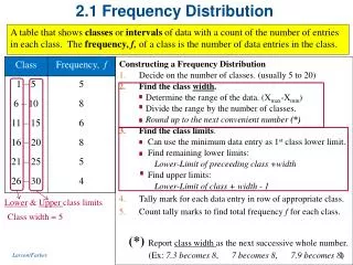
Frequency Distribution I. How Many People Made Each Possible Score? A. This is something I show you for each quiz.
U.S. Distribution of Income Over Time • Share of Income: Richest 1% Poorest 20% 1920 14.4% NA 1970 7.8% 4.2% 2007 18.0% 3.4%
Measurement I. Quantifying and Describing Variables -1 • Four Levels of Measurement • Measures of Central Tendency • Mode • Median • Mean
Measurement I. Quantifying and Describing Variables - 2 DON’T WRITE – JUST READ! We need to review the levels of measurement before continuing. Since you have definitions for the levels of measurement on pages 10-12 of the 300Reader, there is NO REASON to write the following definitions
Four Levels of Precision For Measuring Variables • Nominal Measure: You can put cases into a category, but cannot specify an order or relationship between the categories. • Example: The variable “religion” can take on values such as Catholic, Protestant, Mormon, Jewish, etc.
Four Levels of Precision For Measuring Variables • Ordinal Measure: You can put cases into different categories, and order the categories. • Example: The variable “strength of religious belief” can take on values such as devoutly religious, fairly religious, slightly religious, not religious.
Four Levels of Precision For Measuring Variables • Interval Measure: Not only can you order the categories of the variable, you can specify the difference between any two categories. • Example. The variable “temperature on the Fahrenheit scale” can take on values such as 32 degrees, 74 degrees, 116 degrees.
Four Levels of Precision For Measuring Variables • Ratio Measure: You can order categories, specify the difference between two categories, and the value of zero on the variable represents the absence of the variable. • Example. The variable “annual income” can take on the values of $0, $98,000, or $694,294,129.
Example of a Ratio Measure: Income Inequality The next several slides what groups in the United States, Japan and Sweden think is the actual and fair degree of income inequality between an executive and an auto worker. Since a score of zero equals the absence of income, and the difference between $1 and $2 is the same as between $1,000 and $1,001, we have a ratio level measure.
United States Perceived Fair Income Income Business 15.1/1 15.6/1 Labor 14.8/1 7.2/1 Republicans 13.2/1 11.3/1 Democrats 15.4/1 8.2/1 Youth 13.4/1 6.0/1
Japan Perceived Fair Income Income Business 9.1/1 8.6/1 Labor 10.1/1 4.1/1 Conservative 7.1/1 5.4/1 Party Left Parties 10.3/1 3.7/1
Sweden Perceived Fair Income Income Business 2.4/1 3.5/1 Labor 3.2/1 1.9/1 Conservative/ 2.2/1 2.1/1 Center Party Left Party 3.2/1 1.9/1
Kobe Bryant $24.8 million Paul Gasol $17.8 million Andrew Bynum $13.7 million Lamar Odom $8.2 million Ron Artest $6.3 million Luke Walton $5.2 million Steve Blake $4.0 million Derek Fisher $3.7 million Shannon Brown $2.1 million Matt Barnes $1.7 million Theo Ratliff $1.3 million Joe Smith $1.3 million Devin Ebanks $0.4 million Derrick Caracter $0.4 million Measures of Central Tendency -1
Measures of Central Tendency - 2 • Mode: The most frequently occurring value. • $1.3 million and $0.4 million • Median: The midpoint of the distribution of cases. • 1. Arrange cases in order • 2. If the number of cases is odd, median is the value taken on by the case in the center of the list. • 3. If the number of cases is even, median is the average of the two center values. $3.85 million • (4.0 + 3.7 = 7.7 and 7.7/2 = 3.85)
Measures of Central Tendency - 3 DO NOT WRITE ANY OF THE FORMULAS THAT APPEAR AHEAD! THEY ARE IN THE 300READER AND ONLY APPEAR AHEAD FOR PURPOSES OF DISCUSSION.
Measures of Central Tendency - 4 Mean is the arithmetic average of the values that all the cases take on. Formula: Add up all the values and divide this sum by the number of cases, N. In our Laker example, $6.5 million.
Measures of Central Tendency - 5 Bush Tax Cut Example A. The “Mean” household tax cut under the Bush Tax Cuts is $1,199 while the “Median” household only receives $217. 1. Quite a Difference! 2. 75% of Households Actually Lose Under the Bush Tax Cuts
Measures of Central Tendency - 6 Question: Why can’t the mean tell us everything? Answer: While the mean tells us the average, it does NOT tell us how accurate the mean is when making predictions.
Measures of Dispersion - 1 Thus, we need to know whether the mean occurred because many scores were quite close to the mean or was the mean an average of scores quite different than the mean? This is what measures of dispersion tell us. DON’T WRITE THE FORMULAS AHEAD!!
Measures of Dispersion - 2 The variance is a measure of how spread out cases are, calculated by: Compute the distance from each case to the mean, then square that distance. Find the sum of these squared distances, then divide it by N-1. Lakers: $54.1million.
Measures of Dispersion - 3 The standard deviation is the square root of the variance. For the Laker data, $7.4 million.
Measures of Dispersion - 4 According to page 25 of the 300 Reader, what conclusion should I draw about the dispersion of the Laker data when the mean is 6.5 and the standard deviation is 7.4?
Characteristics of the Normal Distribution -1 It is symmetrical -- Half the cases are to one side of the center; the other half is on the other side. The distribution is single peaked, not bimodal or multi-modal Most of the cases will fall in the center portion of the curve and as values of the variable become more extreme they become less frequent, with “outliers” at each of the “tails” of the distribution few in number.
Characteristics of the Normal Distribution -2 It is only one of many frequency distributions but the one we will focus on for most of this course. The Mean, Median, and Mode are the same. Percentage of cases in any range of the curve can be calculated.
Summarizing Distributions Two key characteristics of a frequency distribution are especially important when summarizing data or when making a prediction from one set of results to another: • Central Tendency • What is in the “Middle”? • What is most common? • What would we use to predict? • Dispersion • How Spread out is the distribution? • What Shape is it?
Appropriate Measures of Central Tendency • Nominal variables Mode • Ordinal variables Median • Interval level variables Mean - If the distribution is normal (median is better with skewed distribution)
Logic of Measures of Dispersion 1 Why not think of dispersion as the difference between the highest and lowest scores?
Logic of Measures of Dispersion 2 If we need a measure based upon all the scores, why not just subtract the mean from each score, add up this total and divide by the total number of scores?
Logic of Measures of Dispersion 3 If the sum of all the deviations from the mean is zero, we could take the absolute value of each deviation from the mean and avoid this problem. So, why don’t we? So, what do we do?
Logic of Measures of Dispersion 4 What is the utility of Tchebysheff’s Theorem?