Download
1 / 27
270 likes | 398 Views
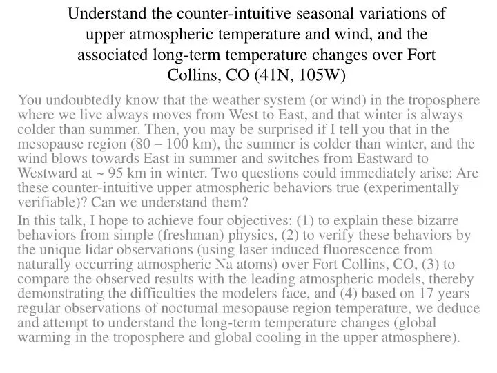
Understand the counter-intuitive seasonal variations of upper atmospheric temperature and wind, and the associated long-term temperature changes over Fort Collins, CO (41N, 105W).

E N D
Understand the counter-intuitive seasonal variations of upper atmospheric temperature and wind, and the associated long-term temperature changes over Fort Collins, CO (41N, 105W) You undoubtedly know that the weather system (or wind) in the troposphere where we live always moves from West to East, and that winter is always colder than summer. Then, you may be surprised if I tell you that in the mesopause region (80 – 100 km), the summer is colder than winter, and the wind blows towards East in summer and switches from Eastward to Westward at ~ 95 km in winter. Two questions could immediately arise: Are these counter-intuitive upper atmospheric behaviors true (experimentally verifiable)? Can we understand them? In this talk, I hope to achieve four objectives: (1) to explain these bizarre behaviors from simple (freshman) physics, (2) to verify these behaviors by the unique lidar observations (using laser induced fluorescence from naturally occurring atmospheric Na atoms) over Fort Collins, CO, (3) to compare the observed results with the leading atmospheric models, thereby demonstrating the difficulties the modelers face, and (4) based on 17 years regular observations of nocturnal mesopause region temperature, we deduce and attempt to understand the long-term temperature changes (global warming in the troposphere and global cooling in the upper atmosphere).
Outline and Conclusions • Introduction: Why necessary? How to measure? • Two unique midlatitudelidar data sets - Four years full-diurnal-cycle TUV observations - Seventeen years nocturnal temperatures • Observed seasonal variations in mesopause region (80 – 110 km) TUV consistent with our qualitative understanding; model-observation difference smaller than differences between models. • Observed cooling trend about 7 times too big if episodic warming in the 1990’s is ignored; it agrees with model prediction if included. • Conclusions
Observing atmospheric layers with active probes XUV UV Radar Gap: 25 – 60 km IR/VIS
a – + Laser induced fluorescence to measure temperature & windT (2-freq) or T-W (3-freq) measurement c • R2-f = Ic / Ia • RT = (I+ + I- ) / 2Ia; RW = (I+ - I- ) / Ia 1nm = 35 cm-1; 1 cm-1 = 30 GHz 1MHz = 0.6m/s; 2MHz ~ 0.3K
2-f and 3-f methods R2-f R2-f = Ic / Ia RT = (I+ + I- ) / 2Ia; RW = (I+ - I- ) / Ia
T (K) Altitude (km) Month Climatology – Two-level Mesopause #m-3 Eight-year Fort Collins climatology of 3.7 km and 1 month smoothed nocturnal temperature (left) and Na density (right) – She et al. GRL 2000
Global Zonal Wind Patterns at Solstice – CIRA ‘86 MLT Mesopause Region Can we understand this zonal wind structure simply? Yes and may be!
How do we understand wind and its structure (cold) ┴ to press. (warm) Motion viewed from turntable in dt, as if acc. by due to a pseudo (Coriolis) force ┴ v to the right: right (left) turn in NH (SH) Why wind blow along isobars? Coriolis “force” make flow right turn on NH, and left turn on SH At rest Rotate c.c.w North pole out ; South pole in
Solar heating and general circulation Forcing: Coriolis “force” and absorption by ground and O3 layer produces zonal winds in troposphere, stratosphere and lower mesosphere: Midlatitude Westly in troposphere: Equator warmer than Poles (summer and winter) → wind towards East Midlatitude Westly in winter stratosphere: Equator warmer than Poles; Ozone → wind towards East Midlatitude Eastly in summer stratosphere: Equator cooler than Poles → wind towards West Big question: Why zonal wind change direction in the MLT, while there is no major heating source in that region?
Gravity wave (GW or buoyancy wave) propagation: filtering and breaking Body force: Winter, West Body force: Summer, East If moving in the same direction, and 0<cW < u, propagation forbidden Adapted from Fig. 3 of Lindzen, JGR (1981).
Waves break, deposit momentum, induce meridional flow East in, West out; Red BF, Green CF • GW propagates upward growing in amplitude, breaks and deposit momentum that applies body force and changes the direction of flow. • The body force (BF) is balanced by the Coriolis force (CF), inducing circulation (meridional drift from SP to WP, and and vertical) cooling summer and warming winter MLT.
No wave can propagate (in medium at rest) outside the shock cone. Wave cannot propagate to the right because 0 < Vw < Vs or 0<cw<us. What if the medium moves with a speed u = us? The source will look stationary on, earth frame, like in this real example Earth frame u>0 cw In the frame of wind, u > 0, the situation may be depicted as: Moving with u us=-u NASA satellite image. Amsterdam Island in the Indian Ocean. December 19, 2005.
Gravity Waves also called buoyancy waves, are waves in the atmosphere propagating against a stratified background state. The restoring force for gravity wave oscillations is the buoyancy force resulting from the displacements of these air parcels from equilibrium. Gravity wave generation by discontinuities: Topography (above example) Wind shear Convection 0400UT Gravity wave observed with Yucca Ridge all sky imager 5/11/2004. Yue et al. NEXRAD echo top height chart, at 0305 UT
Mean-state climatology of mesopause region temperature, zonal and meridional winds Full-diurnal-cycle data set used in this study (10 sets each month on the average) • General seasonal variations of mesopause region temperature and horizontal wind (though counter-intuitive as discussed) has been anticipated, yet different GCMs disagree in predictions. • True mean-state observations with the removal of tidal perturbations are rare or not in existence. To do so require full-diurnal-cycle observations. • With 4-years of 24-hour continuous (full-diurnal-cycle) observations, Yuan et al. (JGR, 2008) have presented results and compared to three leading GCMs (WCCAM3, HAMMONIA and TIME-GCM).
The observed results are in qualitative agreement with our current understanding of the mesopause region thermal and dynamical structure, with two-level mesopause and sharp winter-summer transition, zonal wind switching directions in both summer and winter, as well as “residual” meridional flow from summer pole to winter pole.
The tuning of gravity wave spectra giving rise to different wind filtering could lead to a difference between the different simulations in WACCM3 as large as that between different models. The difference between observation and one model is smaller than those between different models suggests the value of this type of observation.
Temperature Trend: Observed cooling trends from different locations in the mesopause region ranging from 0 to ~10 K/decade. After two decades, the observed trend remains inconclusive.
Long-term variation of nocturnal temperatures Time series at the two-level mesopause (86 km; 99 km)
What variations contain in our data? Annual and semiannual variations, z-dependent Long-term variations: Trend, SC, and episodic response? Pinatubo Response: P(t) = 2/{exp(t0-t)/t1 + exp(t - t0)/t2} with the response amplitude g(z). [She et. al., 1998] Solar response: d(z), in K/SFU [0.05 K/SFU ~ 8 K/SC (11 Y)] with Q(t) being the 81-day smoothed F10.7 solar flux Linear temperature trend, b(z), in K/years Three different analyses with the same data set (1990-2007): 7 P, 11P, and 7PR: Pinatubo response ignored, included and removed.
The solar cycle response in K/SFU (a), and temperature trends in K/decade (b), between 85 and 105km for data sets in different periods: 1990–2001 (open black circles), 1990–2007 (red open/solid squares), 1997–2007 (open blue diamonds), and 1998–2007 (solid blue diamonds).
Same nocturnal mean temperature data (1990 – 1997) used. Comparison between the analyses with “Pinatubo effect” removed (Red) and ignored (Black).
The temperature trend using lidar data (1990 – 2007) and ignore the volcanic response yields cooling trend of as much as 6.8 K/decade. With a Pinatubo term included, the observed negative linear trend between 85 and 100 km peaks at 91 km with a value of ~1.5 K/decade, and it turns positive at ~ 102 km. We observed an insignificant cooling trend of 0.28 K/decade at 87 km. This trend result compares favorably with the SMLTM and HAMMONIA model predictions. Lidar Trend compares with model predictions F-11P and F-7PR in agreement with different error bars
Response to Mt. Pinatubo Eruption: mesopause vs. global-mean surface temperatures Can we believe the Pinatubo response that delayed 1.5 Y and lingered 7 years? A recent analysis of long-term climate variability of global-mean surfacetemperatures by Thompson et al. (J. Climatr, 2009), revealed an episodic cooling after Mt. Pinatubo eruption also with ~1.5 year delayed peak response, which is deduced to have a recovery time of ~7 years (blure dots, *-50)
Conclusion • The CSU Na lidar has begun regular mesopause region observations of nocturnal temperature and Na density since 1990; of full-diurnal cycle DNa, T, U, V since 2002; and, in addition, of zonal momentum flux since September 2006. • The 17 years (1990-2007) nocturnal temperatures are used to deduce an episodic response in the 1990’s following Mt. Pinatubo eruption, solar cycle effect and temperature trends, with the deduced trends in agreement with model predictions. • The 4 years full diurnal cycle T, U, V observations have been used to deduce tidal-removed climatologies. The observed TUV climatology is in agreement with our current understanding of the mesopause region; when compared with three leading GCMs, the observation-model differences appear to be smaller than the differences between models.
Krueger and She (2009): Seasonal variation of T, trend, solar: Based on1990-2007 “Pinatubo removed” nocturnal temperatures
First 80 hours of continuous observation; She et al. (GRL, 2003) Comparison between means with night- and day-only data, all 80 hours, and harmonic fit reveal the aliasing in the determination of mean-state from data less than 24-hour long and with data gap.