Download
1 / 28
280 likes | 457 Views
Introduction to Control: How Its Done In Robotics. R. Lindeke, Ph. D. ME 4135. Remembering the Motion Models:. As we found using the L-E approach, the Required Joint Torque is:. Dynamical Manipulator Inertial Tensor – a function of position and acceleration.

E N D
Introduction to Control: How Its Done In Robotics R. Lindeke, Ph. D. ME 4135
Remembering the Motion Models: • As we found using the L-E approach, the Required Joint Torque is: Dynamical Manipulator Inertial Tensor – a function of position and acceleration Coupled joint effects (centrifugal and coriolis) issues due to multiple moving joints Gravitational Effects Frictional Effect due to Joint/Link movement
Lets simplify the model (a Bit) • This torque model is a 2nd order one (in position) lets look at it as a velocity model rather than positional one then it becomes a system of highly coupled 1st order differential equations • We will then isolate Acceleration terms (acceleration is the 1st derivative of velocity)
Considering Control: • Each Link’s torque is influenced by each other links motion • We say that the links are highly coupled • Solution then suggests that control should come from a simultaneous solution of these torques • We will model the solution as a “State Space” design and try to balance the torque-in with positional control-out – the most common way it is done! • But we could also use ‘force control’ to solve the control problem!
State Space Approach • The State Space General Model feeds out positional kinematics based on the “torque (power) demand” input • Notice: 1/s is the Laplace transform of a unit step (torque) impulse • As you remember, Laplace transforms convert linear differential equation sets into algebraic equation sets • once solved we need to do inverse Laplace transforms to return to torque/position space • In LaPlace models, S is a complex variable!
Ultimately how do we know How much Torque to specify – and if we are ‘In Control’ • In robots with moving joints, we set targets for motion • We sense motion at the joint level (using kinesethic sensors) • We study differences between where we are and where we’re going as a “Feedback” (ie. servo) error • Control means that we try to minimize error (make error go to zero) when we move toward a new location
Setting up a Real Control • We will (start) by using positional error to drive our torque devices • This simple model is called a PE (proportional error) controller
PE Controller: • To a 1st approximation, = Km*I • Torque is proportional to motor current • And the Torque required is a function of ‘Inertial’ (Acceleration) and ‘Friction’ (velocity) effects as suggested by our L-E models
Setting up a “Control Law” • We will use the positional error (as drawn in the state model) to develop our torque control • We say then for PE control: • Here, kpe is a “gain” term that guarantees sufficient current will be generated to develop appropriate torque based on observed positional error
Using this Control Type: • It is a representation of the physical system of a mass on a spring! • We say afer setting our target as a ‘zero goal’ that: a is a function of the servo feedback as a function of time!
Examining this ‘solution’: • The 1st term is a damping term for the motion • The systems ‘natural frequency’ is given by:
Studying the solution: • If (F2/4kpe)> J we are ‘over damped’ and the system will never quite reach its target considering “reasonable time” • If (F2/4kpe)= J we are ‘critically damped’ giving the system ideal behavior • If (F2/4kpe)< J we are ‘under damped’ and the system will over-shoot and oscillate about our target at the system’s natural frequency – a dangerous situation in robotics!
These behaviors make sense (physically!): • Under High Friction Conditions (over damped): • A system is hard to start but easy to stop • With High Moment of Inertia Conditions (under damped): • A system is hard to start and it is hard to stop leading to overshoot and possibly one that oscillates about the target ‘forever’
Problems with PE Control: • First the so-called “Steady-State” error – the torque goes to zero when the target is hit! • Secondly, we may be out of balance – the GAIN is not meeting our Inertial vs. Friction balance leading to overshoot or undershoot • Typically we will add a term to our model to react to increasing speed so we minimize overshoot
Dealing With Steady State Zero Error • This is a gravitational issue: we must add an ‘L’ or gravitational term back to our Torque control model • Gravitational input is positionally controlled: • L = -g (M1r1 + M2R)* Cos() For a R Manipulator with a payload on M2
Solving the Overshoot Problem: • Lets expand our control law: • We should include a term that reacts to the velocity of the link – • But velocity is the derivative of the position • We will call this a proportional – derivative controller (PD Control)
Solving the PD Model: • Remembering:
Effect of Derivative Term: • It is observed to be a form of “Active Friction” • It tends to slow down the link as it moves faster when high errors (being far from goal) are observed • Thus it can be thought of as a brake on the motion • It is a component that anticipates changes and provides very fast response to these changes
Taking Care of Trouble: • We add an integrator to the model • To damp out oscillations from over shoot • To control effects due to environmental perturbations • To damp out Wild data gyrations – typically due to encoder errors • This leads to a model of control:
Developing Optimal Control • PID is most often found in the systems Arm Joints • The components of Torque are functions of POSE meaning the Jeq and Feq as well as L factors change as one observes the robot moving throughout the work envelope • We achieve control with kpe, kd and ki • if they are fixed values, we can expect critically damped control at only a single (or very few) position(s)
What is done: • We operate off critical PID on arm joints and PD w/ gravitational compensation for remote and wrist joints • Most controls use a form of adaptive control • Tables of gains applicable over certain geometries with automatic changes as the manipulator moves about the work envelope • We swap in and out the gain values such that we minimize energy consumed by the drive:
Another Idea: • Develop a Performance Index (PI) that judges controller stability • This PI is an external measurement scheme that using logic and comparisons between desired and actual performance then adjusts the model
Thus Ends our Introductory Studies of “Robotics & Controls” • This is a rich and deep field of applied Mechanical and Industrial Engineering • While we have deeply explored some topics, others have only been scanned • I wish you well as you move forward in your lifelong exploration of “AUTOMATION” and its myriad of supporting technologies • I sincerely hope that you have all learned something of this fascinating field and that these lessons will prove to be valuable in your careers!