Download

1 / 56
580 likes | 849 Views
Lecture 6 Power and Sample Size in Linear Mixed Effects Models. Ziad Taib Biostatistics, AZ MV, CTH May 2011. 1. Date. Outline of lecture 6. Generalities Power and sample size under linear mixed model assumption Example 1: The rat data Estimating sample size using simulations

E N D
Lecture 6Power and Sample Size in Linear Mixed Effects Models Ziad Taib Biostatistics, AZ MV, CTH May 2011 1 Date
Outline of lecture 6 • Generalities • Power and sample size under linear mixed model assumption • Example 1: The rat data • Estimating sample size using simulations • Example 2: COPD Name, department
(from ICH-E9) “The number of subjects in a clinical study should always be large enough to provide a reliable answer to the question(s) addressed.” “The sample size is usually determined by the primary objective of the trial.” “ Sample size calculation should be explicitly mentioned in the protocol .”
Power and sample size Suppose we want to test if a drug is better than placebo, or if a higher dose is better than a lower dose. Sample size: How many patients should we include in our clinical trial, to give ourselves a good chance of detecting any effects of the drug? Power: Assuming that the drug has an effect, what is the probability that our clinical trial will give a significant result?
Sample Size and Power Sample size is contingent on design, analysis plan, and outcome With the wrong sample size, you will either Not be able to make conclusions because the study is “underpowered” Waste time and money because your study is larger than it needed to be to answer the question of interest
Sample Size and Power With wrong sample size, you might have problems interpreting your result: Did I not find a significant result because the treatment does not work, or because my sample size is too small? Did the treatment REALLY work, or is the effect I saw too small to warrant further consideration of this treatment? Issue of CLINICAL versus STATISTICAL significance
Sample Size and Power Sample size ALWAYS requires the scientist/investigator to make some assumptions How much better do you expect the experimental therapy group to perform than the standard therapy groups? How much variability do we expect in measurements? What would be a clinically relevant improvement? The statistician alone CANNOT tell what these numbers should be. It is the responsibility of the scientist/clinical investigators to help in defining these parameters.
Errors with Hypothesis Testing Reject H ccept H A A 0 Ho true E = C OK Type I error Ho false Type II error OK E C ≠ Ho: E=C (ineffective) HA: E≠C (effective)
Type I Error Probability of Type I error = significance levelor a level Value needs to be pre-specified in the protocol and should be small Explicit guidance from regulatory authorities, e.g. 0.05 One-sided or two-sided ? Ho: drug ineffective vs.HA: drug effective Concluding for alternative hypothesis while null-hypothesis is true(false positive)
Type II Error Probability of Type II error = b level Value to be chosen by the sponsor, and should be small No explicit guidance from regulatory authorities, e.g. 0.20, or 0.10 Power = 1 - Type II error rate. Typical values 0.80 or 0.90 Concluding for null-hypothesis while alternative hypothesis is true (false negative)
Sample Size Calculation Following items should be specified a primary variable the statistical test method the null hypothesis; the alternative hypothesis; the study design the Type I error the Type II error way how to deal with treatment withdrawals
Power calculations in practice • In the planning and development stage of an experiment, a sample size calculation is a critical step. In controlled clinical trials, sample size calculation is required to maintain specific statistical power (i.e. 80% power) for the study. Not surprisingly, there are many software packages (i.e. nQuery, PASS, StudySize etc) which perform sample size calculation for certain statistical tests. However, such software packages are not available for sample size calculations for complex designs and complex statistical analysis methods. Name, department
Power Calculations Under Linear Mixed Models • In the following, we will discuss the design of longitudinal studies. • We will briefly discuss how power calculations can be performed based on linear mixed models. • In practice longitudinal experiments often do not yield the amount of information hoped for at the design stage, due to dropout. This results in realized experiments with (possibly much) less power than originally planned. • We will discuss how expected dropout can be taken into account in sample-size calculations. The basic idea behind this is that two designs with equal power under the absence of dropout are not necessarily equally likely to yield realized experiments with high power. • The main question then is how to design experiments with minimal risk of huge losses in efficiency due to dropout. • The above is illustrated in the context of the rat experiment. Name, department
Power Calculations Under Linear Mixed Models • We have discussed inference for the marginal linear mixed model. Several testing procedures were discussed, including • approximate Wald tests, • approximate t-tests, • approximate F -tests, • and likelihood ratio tests (based on ML as well as REML estimation), for the fixed effects as well as for the variance components in the model. • Obviously, any of these testing procedures can be used in power calculations. . Name, department
Power Calculations Under Linear Mixed Models • Unfortunately, the distribution of many of the corresponding test statistics is only known under the null hypothesis. • In practice, this means that if such tests are to be used in sample-size calculations, extensive simulations would be required. • One then would have to • sample data sets under the alternative hypothesis of interest, • analyze each of them using the selected testing procedure, • and estimate the probability of correctly rejecting the null hypothesis. • Finally, this whole procedure would have to be repeated for every new design under consideration
Power Calculations Under Linear Mixed Models • Assume we are interested in a general linear hypothesis of the forms • Then we can use the (Under H0) approximately F-distributed statistic
Power Calculations Under Linear Mixed Models • Helmert (1992) reports that under the alternative hypothesis HA , the distribution of F can also be approximated by an F-distribution, now with rank(L) and Sini - rank[X|Z] degrees of freedom and with non-centrality parameter: • With notation as in previous lectures
The rat data • The hypothesis of primary interest is H0 : no effect, which turns out to be non-significant using an approximate Wald statistic (p=0.0987). A similar result (p=0.1010) is obtained using an approximate F -test, with Satterthwaite approximation for the denominator degrees of freedom. We conclude from this that there is little evidence for any treatment effects. However, the power for detecting the observed differences at the 5% level of significance and calculated using the F -approximation described in the previous section is as low as 56%. Name, department
Note that, this rat experiment suffers from a severe degree of dropout, since many rats do not survive anesthesia needed to measure the outcome. Indeed, although 50 rats have been randomized at the start of the experiment, only 22 of them survived the 6 first measurements, so measurements on only 22 rats are available in the way anticipated at the design stage. For example, at the second occasion (age = 60 days), only 46 rats were available, implying that for 4 rats, only 1 measurement has been recorded. As can be expected, this high dropout rate inevitably leads to severe losses in efficiency of the statistical inferential procedures. Indeed, if no dropout had occurred (i.e., if all 50 rats would have withstood the 7 measurements), the power for detecting the observed differences at the 5% level of significance would have been 74%, rather than the 56% previously reported for the realized experiment. Could we have used a better design? Name, department
Conclusion • In the rat example, dropout was not entirely unexpected since it is inherently related to the way the response of interest is actually measured (anesthesia cannot be avoided) and should therefore have been taken into account at the design stage. Therefore we need methods for the design of longitudinal experiments, when dropout is to be expected. We will discuss such an approach and apply it to the rat data. Name, department
Power Calculations When Dropouts are to Be Expected • In order to fully understand how the dropout process can be taken into account at the design stage, we first investigate how it affects the power of a realized experiment. • Note that the power of the above F -test not only depends on the true parameter values b, D, and Sibut also on the covariates Xi and Zi. Usually, in designed experiments, many subjects will have the same covariates, such that there are only a small number of different sets (Xi ,Zi ). Name, department
For the rat data, all 15 rats in the control group have Xi and Ziequal to Name, department
However, due to the dropout mechanism, the above matrices have been realized for only four of them. Indeed, for a rat that drops out early, say at the kth occasion, the realized design matrices equal the first k rows of the above planned matrices; that is, Name, department
Note that the number of rats that drop out at each occasion is a realization of the stochastic dropout process, from which it follows that the power of the realized experiment is also a realization of a random variable, the distribution of which depends on the planned design and on the dropout process. From now on, we will denote this random power function by P. • Since, in the presence of dropout, the power Pbecomes a stochastic variable, it is not obvious how two different designs with two different associated power functions P1 and P2should be compared in practice. Several criteria can be used, such as the average power, E(P1), the median power, median(P1), the risk of having a final analysis with power less than for example 70%, P (P < 70%), and so forth. Name, department
Note that all of the above criteria are based on only one specific aspect of the distribution of P1. A criterion which takes into account the full distribution selects the second design over the first one if P1 is stochastically smaller than P2 , which is defined as (Lehmann and D’Abrera 1975, p. 66) P1is stochastically smaller than P2 P (P1 <p ) > P (P2 <p ) for all p This means that, for any power value p, the risk of ending up with a final analysis with power less than p is smaller for the second design than for the first design. Name, department
Obviously, if the above criterion is to be used, one needs to assess the complete power distribution function for all designs which are to be compared. We propose doing this via sampling methods in which, for each design under consideration, a large number of realized values ps , s=1,...,S, are sampled from Pand used to construct the empirical distribution function below where I[A] equals one if A is true and zero otherwise. Name, department
As indicated above, sampling from Pactually comes down to sampling realized values and constructing all necessary realized matrices Xj[k]and Zj[k]. One then can easily calculate the implied non-centrality parameter d and the appropriate numbers of degrees of freedom for the F-statistic, from which a realized power follows. • It should be emphasized that the above approach is not restricted to any particular statistical test. The idea of sampling designs under specific dropout patterns is applicable for any testing procedure, as long as it remains possible to evaluate the power associated to each realized design. Name, department
Note also that the only additional information needed, in comparison to classical power analyses, are the vectors pjof marginal dropout probabilitiespj,k . This does not require full knowledge of the underlying dropout process. • We only need to make assumptions about the dropout rate at each occasion where observations are designed to be taken. • For example, we do not need to know whether the dropout mechanism is “completely at random” or “at random”.
Still, we have to assume that dropout is “not informative” in the sense that it does not depend on the response values which would have been recorded if no dropout had occurred, since otherwise our final analysis based on the linear mixed model would not yield valid results (see Section 15.8 and Chapter 21). • Finally, the proposed method can be used in combination with techniques, such as those proposed by Helms (1992), which would allow the costs of performing the designs under consideration to be taken into account. This could yield less costly experiments with minimal risk of large efficiency losses due to dropout. This will not be explored any further here. Name, department
The rat data • Observed conditional dropout rates at each occasion, for all treatment groups simultaneously. • Age (days): • Observed rate: • Based on the data we assume that each time a rat is anesthetized, there is about 12% chance that the rat will not survive anesthesia, independent of the treatment. • All calculations are done under the assumption that the true parameter values are given by earlier estimates and all simulated power distributions are based on 1000 draws from the correct distribution. Name, department
Since, at each occasion, rats may die, it seems natural to reduce the number of occasions at which measurements are taken. We have therefore simulated the power distribution of four designs in which the number of rats assigned to each treatment group is the same as in the original experiment, but the planned number of measurements per subject is seven, four, three, and two, respectively. • These are the designs A to D in the table below. Note that design A is the design used in the original rat experiment. The simulated power distributions are shown in the figure. Name, department
Rat Data. Summary of the designs compared in the simulation study when varying group sizes • Occasions Number of subjects Power if Design Age (days) (M ,M ,M ) no dropout A 50-60-70-80-90-100-110 (15, 18, 17) 0.74 B 50-70-90-110 (15, 18, 17) 0.63 C 50-80-110 (15, 18, 17) 0.59 D 50-110 (15, 18, 17) 0.53 E 50-70-90-110 (22, 22, 22) 0.74 F 50-80-110 (24, 24, 24) 0.74 G 50-110 (27, 27, 27)0.75 H 50-60-110 (26, 26, 26) 0.74 I 50-100-110 (20, 20, 20) 0.73 A: Original design Name, department
Comparison of the simulated power distributions for designs with seven, four, three, or two measurements per rat, with equal number of rats in each design (designs A, B, C, and D, respectively), under the assumption of constant dropout rate equal to 12%. The vertical dashed line corresponds to the power which was realized in the original rat experiment (56%). 1 0.80 Design A Design B P(Power ≤ p) Design C Design D 0 p 0.5 0.6 0.3 56% P(PA <0.56)=0.80 Name, department
First, note that the solid line is an estimate for the power function of the originally designed rat experiment under the assumption of constant dropout probability equal to 12%. • It shows that there was more than 80% chance for the final analysis to have realized power less than the 56% which was observed in the actual experiment. • Comparing the four designs under consideration, we observe that the risk ofhigh power losses increases as the planned number of measurements per subject decreases. • On the other hand, it should be emphasized that the four designs are, strictly speaking, not comparable in the sense that, in the absence of dropout, they have very different powers ranging from 74% for design A to only 53% for design D.
Designs E, F, and G are the same as designs B, C, and D, but with sample sizes such that their power is approximately the same as the power of design A, in the absence of dropout. • The simulated power distributions are shown below. The figure suggests that A > E > F > G , from which it follows that, in practice, the design in which subjects are measured only at the beginning and at the end of the study is to be preferred, under the assumed dropout process. • The above can be explained by the fact that the probability for surviving up to the age of 110 days is almost twice as high for design G (88%) as for the original design (46%). • Note also that the parameters of interest [b1 , b2, and b3] are slopes in a linear model such that two measurements are sufficient for the parameters to be estimable. On the other hand, design G does not allow testing for possible nonlinearities in the average evolutions. Name, department
PA <PE <PF <PG Unlikely with power less than 0.56 for the new designs) 1 Design E Design A 0.80 Design F P(Power ≤ p) Design G p 0 0.5 0.6 0.3 56% Date P(PA <0.56)=0.80
Comments • Note that the above results fully rely on the assumed linear mixed model. For example, the simulation results show that design G, with only two observations per subject, is to be preferred over designs A, E, and F, with more than two observations scheduled for each subject. • Obviously, the assumption of linearity is crucial here, and design G will not allow testing for nonlinearities. Hence, when interest would be in providing support for the used model, more simulations would be needed comparing the behavior of different designs under different models for the outcome under consideration, and design G should no longer be taken into account. • As for any sample-size calculation, it would be advisable to perform some informal sensitivity analysis to investigate the impact of model assumptions and imputed parameter values on the final results. Name, department
Example: Estimating the sample size needed in a trial for chronic pulmonary diseases • Chronic pulmonary diseases (such as Chronic Obstructive Pulmonary Disease – COPD) concern the development of emphysema. It is a slow progression over many years and the assessment of drug efficacy requires the observation of large numbers of patients for a long period of time. Recently, lung densitometry (measuring the lung density through CT scan) considered for assessing the lung tissue loss over time in patients with emphysema. • A clinical trial with lung densitometry as an endpoint is typically designed as a longitudinal study with repeated measurements at fixed time intervals. Since lung density measurements are closely correlated with lung volume (inspiration level), it is important to include lung volume measurements in statistical analyses as a longitudinal covariate. Lung volume is normally measured at the same time as the lung density is measured. Name, department
The clinical efficacy can be assessed by comparing the progression of lung density loss between two treatment groups using a random coefficient model – a longitudinal linear mixed model with a random intercept and slope. In planning the clinical trial with such complex statistical analyses, the calculation of the sample size required to achieve a given power to detect a specified treatment difference is an important, often complex issue. • In this example, an empirical approach is used to calculate the sample size by simulating trajectories of lung density and lung volume using SAS. We present step-by-step details for sample size calculation through simulation, and discuss the pros and cons of this approach. (1) Name, department
Here Yijis the efficacy endpoint (i.e. lung density) measurement for subject i = 1, 2,…, n, at fixed time point j = 1, 2, …, K. • TRT is an indicator of subject i’s treatment group (i.e. TRT=1 for active drug; TRT=0 for placebo). • COVij is a longitudinal covariate (i.e. logarithm of lung volume) for subject i = 1, 2,…, n, at fixed time point j = 1, 2, …, K. • Here b0 and b2 are subject-specific random effects for the intercept and slope, respectively, which are from a normal distribution with mean 0 and variance σ02 and σ02, respectively. • εijis the random error from a normal distribution with mean 0 and variance σ2. • The regression parameters β0, β1, β2, β3, and β4 are the fixed effects for intercept, treatment, time, covariate and interaction of treatment and time respectively. • Here we assume that the benefits can be assessed quantitatively by comparing the slopes of lung density trajectories for the two treatment groups. This quantity is captured by β4.
Sample Size Estimation Using Simulations • In the model, β4is typically of interest. There is no direct mathematical formula to calculate the sample size for a given statistical power (i.e. 80%) to test the null hypothesis: β4=0 with a specified type I error (i.e. α=0.05). • One approach to calculate the sample size for a given power is through the simulation.
Simulating the response • Assume we know the parameters (β0, β1, β2, β3, and β4, and σ02 and σ02) from either history data, previous clinical trials or meaningful clinical differences we want to test, the study design in terms of number of time points (K) and fixed time intervals (TIME), and the longitudinal covariate COVij. • For a fixed equal sample size n for each treatment, the trajectories of efficacy measurement Yij (i.e. lung density) for the n subjects can be simulated through the model for each treatment group. • Then, perform a statistical test on β4 =0 by using the SAS Proc MIXED on the simulated data set, and record whether the p-value < 0.05.
In order to simulate the trajectories of Yij, it is necessary to simulate the trajectories of longitudinal covariate COVij. Assume COVij is from a linear model regressing against time with a random intercept • Where γ0 and γ1 are the fixed intercept and slope respectively; r0 and εij are from a normal distribution with mean 0 and variance d12 and d22, respectively. If we know the parameters (γ0,γ1 , d12 and d22 ) from history data or previous clinical trials for the study population, it will be simple to simulate the trajectories of the longitudinal covariate COVij by using SAS random generating functions. (2) Name, department
In detail, a sample size can be determined for the models above through the following steps: 1. Obtain the pre-specified parameters through either history data, previous clinical trials or meaningful clinical difference to be tested from clinicians 2. Specify a desired statistical power (i.e. 80%) and a type-1 error rate (i.e. 5%) 3. Simulate trajectories of efficacy measurement (i.e. lung density) and longitudinal covariate (i.e. logarithm of lung volume) for a fixed sample size (n) of subjects within each treatment arm • A. Trajectories of longitudinal covariate (i.e. logarithm of lung volume) are simulated through model (2) • B. Trajectories of efficacy measurement (i.e. lung density) are simulated through model (1)
4. Perform the statistical test on β4=0using the SAS Proc MIXED based on the simulated data set. Record whether a p-value < 0.05 was obtained 5. Repeat steps 3 and 4 M (i.e. M=1000) timesand calculate the statistical power for the fixed sample size 6. Repeat steps 3 - 5 for various values of n. Stop when desired statistical power is obtained Name, department
The sample code to perform the test is as follow: proc mixed data = data; class id trt; model y = trt time trt*time cov / solution; random intercept time/ subject = id type = un; run; • For the fixed sample size n per treatment group, simulate M (i.e. M=1000) times and the proportion of significant tests of β4 =0 among the total M simulations is the statistical power for the sample size n per treatment group. Then, adjust the sample size n to achieve desirable statistical power.
Example of a Simulation • Assume there are two treatment groups (active vs. placebo) in a study design. The efficacy endpoint along with the longitudinal covariate will be measured at K=4 time points at baseline, 1 year, 2 years and 3 years. All corresponding parameters specified in model (1) and (2) could be obtained either through historical data, previous clinical trials or meaningful clinical difference to be tested from clinicians. For purpose of simulation, they are randomly selected and specified as below: Name, department
The summary of statistical power for a given sample size per treatment based on M = 1000 simulated data sets is listed below: • Therefore, a sample size 45 per treatment arm has an estimated statistical 80% power to detect the treatment slope difference of 0.7 in a random coefficient model for the study design above. Name, department
Conclusions and Discussion • As described above, it is possible to perform sample size calculations for a random coefficient model using simulation techniques and SAS. • It is also straightforward to extend the simulation frame to other linear mixed models (LMM) or generalized linear mixed models (GLMM). • Other extensions: multiple treatment groups (i.e. treatment groups greater than 2), unequal sample size among treatment groups (i.e. 2:1 for active vs. placebo) etc. • For an active-controlled trial, it is usually of interest to test non-inferiority of test drug compared to active-control.