Download
1 / 22
220 likes | 256 Views
Determining a Distribution – histogram approach. One approach to distribution fitting that is visual/intuitive is: Convert collected data d to a histogram ( Next slide starts details the histogram representation ) Notes: Histograms often visually suggest/infer a well-known pmf .

E N D
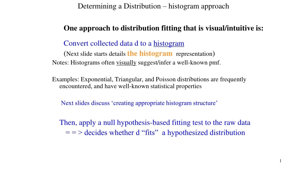
Determining a Distribution – histogram approach One approach to distribution fitting that is visual/intuitive is: Convert collected data d to a histogram (Next slide starts details the histogram representation) Notes: Histograms often visually suggest/infer a well-known pmf. Examples: Exponential, Triangular, and Poisson distributions are frequently encountered, and have well-known statistical properties Next slides discuss ‘creating appropriate histogram structure’ Then, apply a null hypothesis-based fitting test to the raw data = = > decides whether d “fits” a hypothesized distribution
A Ragged histogram (Fig (1) Original Data - Too Ragged – Alternating between domain intervals with 1) empty and 2) well-populated frequencies – shape of section for large domain values (x < 4, and x > 12) unclear {most buckets have minimal population} Comparing Sample Histogram shapes (Source data unspecified) – 1 of 3
A Coarse histogram (Fig (2) Combining adjacent cells - too Coarse – concentrated domain intervals with 1) no vs. 2) well-populated frequencies – Overall shape unclear – at a macro level, many distributions look something like this Comparing Sample Histogram shapes (Source data unspecified) – 2 of 3
An appropriate histogram (Fig (3) Combining adjacent cells – Appropriate – each multi-cell bucket (such as 0-5 or 6-15), etc. is well-populated ; entire histogram shape is evident; {all buckets in the range have content (no empty buckets}; Comparing Sample Histogram shapes (Source data unspecified) – 3 of 3
Discrete Data Example – Example from: Section 9.5, p 342 ofEdition 4, ‘Discrete-Event System Simulation’, by Banks, Carson, et al, Prentice Hall The number of vehicles arriving at the northwest corner of an intersection in a 5-minute period between 7:00 a.m. and 7:05 a.m. was monitored for five workdays over a 20-week period. The table (next slide) shows the resulting data. == > Data set “d” consists of 20*5 = 100 sample values. When d is represented as a frequency distribution table (next slide), The first entry (0,12) in the table indicates there were 12 5-minute periods during which novehicles arrived; The second entry (1,10) indicates there were 10 5-minute periods during which one vehicle arrived, etc. The discrete random variable X in this scenario represents “the number of vehicle arrivals in any 5-minute interval on a random day” The problem is to determine the distribution followed by the X values.
Discrete Data Example (cont.) Arrivals Arrivals per Period Frequency per Period Frequency 0 12 6 7 1 10 7 5 2 19 8 5 3 17 9 3 4 10 10 3 5 8 11 1 Table – Since X is a discrete variable, and since there is sufficient data, the histogram can have a cell for each possible value in the range of data. = > sufficient data reveal relative probabilities more fairly vs. lack of data The resulting histogram is shown in the next slide.
Histogram - Distribution of Number of arrivals per period Number of arrivals over 5-minute intervals - Discrete data example (cont.)
Distribution Fitting Iteration “Fitting” is the process of (iteratively) converging to selection of one particular distribution family and family member parameters that represents d well. Example: if d seems to be Poisson distributed, then this is the distribution family, but as yet, the specific pmf from this family is not determined. Statistics obtained from d will determine the parameters of ONE family member that becomes the candidate distributionpmf Generally, there are 2 major steps to fitting: • Determine appropriate distribution Family F and Parameters in F that determine one specific distribution candidate D • Perform a statistics-based validation of D
Distribution Fitting Iteration The general Multi-step fit algorithm is outlined in posted document: RawDataFitting.doc Goodness-of-Fit Tests For the a) Chi-Square test (covered in this course) and b) Kolmogorov-Smirnov (aka KS) test (not covered in this course): Each Test can evaluate a null hypotheses about whether a distribution of raw data “fits” a hypothesized distribution We will review the concept of a Null Hypothesis soon Next = => the Chi-Square significance test for distribution fitting
The test evaluates how likely the observation’s values would be, assuming the null hypothesis is true. This test is valid for large sample sizes, for both discrete and continuous distributions when parameters are estimated by maximum likelihood. The test procedure begins by arrangingn observations into k class intervals or cells. Then, calculate “test statistic” --- (Eq 5) Oi the observed frequency in the ith class interval (that is, the frequency of xi), and Eiexpected frequency (computed using hypothesized distribution) in ith class interval. Principle: if Oi and Ei are “close”, ith summand of (when expanded out) is a value that should be small = => total test statistic value should thus be relatively small if the data sample “fits” the theoretical distribution Chi-Square has diverse applications (not just distribution fitting), such as: • whether there is significant difference between observed Oi and expected Ei values • iid testing: whether a sequence of random variable values are independent • computer security: whether decryption Dd of given encrypted data De succeeded Chi-Square Test
The hypotheses are: H0: random variable, X, conforms to the distribution assumption with parameter(s) given by parameter estimate(s); This is the Null hypothesis H1: random variable X, does not conform to the distribution The critical value is found in many web references Null hypothesis, H0, is rejected if (see Slide#19) Goodness-of-Fit - Chi-Square Test (cont.) Given a Chi-Square test statistic for sample size n of random variable X. Next, define a null hypothesis and how to test its validity.
Poisson as a representative discrete distribution Example of a typical Poisson distribution, for one mean value a Recall that: The informal (and intuitive) start is to choose a hypothesized classical (well-studied and tabulated) distribution based on the shape of the histogram formed from the collected data.
Goodness-of-Fit Tests - Chi-Square Test (cont.) Example: Chi-Square test applied to Poisson distribution Assumption In traffic example, the vehicle arrival data were analyzed. Since the histogram of the data, shown in Figure 2 appeared to follow a Poisson distribution, parameter estimate, a = 3.64 = x^ = mean of arrivals per observation was determined. (Review the frequency formatted tabulation of the data) Thus, the following hypotheses are formed: The random variable X is: number of vehicles arriving in the intersection in a given 5-minute interval on some workday H0: X is Poisson distributed H1: X is not Poisson distributed
Goodness-of-Fit TestsChi-Square Test (cont.) pmf for Poisson distribution of random variable x with parameter a is: ì(e-aaxi) / xi! , xi = 0, 1, 2 ... p(xi)=í (Eq 6) î0 , otherwise For a = 3.64, the probabilities associated with various values of x are obtained by the equation with the following results. Notice “twin peaks” p(0) = 0.026p(3) = 0.211 p(6) = 0.085 p(9) = 0.008 p(1) = 0.096 p(4) = 0.192 p(7) = 0.044 p(10) = 0.003 p(2) = 0.174 p(5) = 0.140 p(8) = 0.020 p(11) = 0.001
python example: evaluating terms Ei of the Chi-Square fit - 1 of 2 """ chisquareCalcs_s19.py - CSC148 Poisson pmf & Chi-Square Ei calculations Variable names use terminolgy related to the Chi-Square distribution fit """ import math numberOfClasses = int(input("Number of Classes: ")) OiFrequencyMean = float(input("Mean of the class frequencies: ")) sumOfxiFrequencies = int(input("sum of the class frequencies: ")) print("Chi-Square class values calculations tool \n") # The expected Poisson pmf pi values for user-input parameters print("The pmf values for pi = prob(X=xi), xi=0,1,2, ..., assuming NON-combined classes") for xi in range (numberOfClasses): print("p"+str(xi), " is: ",(math.exp(-OiFrequencyMean)*OiFrequencyMean**xi )/math.factorial(xi) ) # The expected Ei values print(“ \nTheEi values for classes E1, E2, etc.") for xi in range (numberOfClasses): print("E"+str(xi), " is: ",sumOfxiFrequencies*(math.exp(-OiFrequencyMean)*OiFrequencyMean**xi )/math.factorial(xi)) = = > Execution results on next Slide Source file at: /gaia/home/faculty/mitchell/simpy3demos/chisquareCalcs_f19.py
python example: evaluating terms Ei of the Chi-Square fit – 2 of 2 Results: ============ RESTART: C:/Users/bill/148_f19/chisquareCalcs_s19.py ============ Number of Classes: 12 Mean of the class frequencies: 3.64 sum of the class frequencies: 100 Chi-Square class values calculations tool The pmf values for pi = prob(X=xi), xi=0,1,2, ..., assuming NON-combined classes p0 is: 0.02625234396568796 p1 is: 0.09555853203510419 p2 is: 0.17391652830388962 p3 is: 0.2110187210087194 p4 is: 0.19202703611793467 p5 is: 0.13979568229385644 p6 is: 0.08480938059160625 p7 is: 0.04410087790763525 p8 is: 0.02006589944797404 p9 is: 0.008115541554513944 p10 is: 0.0029540571258430764 p11 is: 0.0009775243580062542 The Ei values for classes E1, E2, etc. E0 is: 2.6252343965687963 E1 is: 9.555853203510418 E2 is: 17.391652830388963 E3 is: 21.10187210087194 E4 is: 19.202703611793467 E5 is: 13.979568229385645 E6 is: 8.480938059160625 E7 is: 4.410087790763526 E8 is: 2.006589944797404 E9 is: 0.8115541554513944 E10 is: 0.29540571258430764 E11 is: 0.09775243580062543 >>>
Chi-Square Test (cont.) – RESUME traffic example - Topic: Combining classes1) Ei = n*pi; Ei has factor n; expected frequency depends proportionally on sample size; pi =prob(X=xi), so the frequency of xi occurring in sample size n is: n*pi = 100*pi.2) Bracketed values combine >=2 classes into 1 class => Details on next slide Observed Frequency, Expected Frequency, (Oi - Ei)2 / Ei xi Oi n*pi=Ei 0 12 2.67.87 1 10 22 9.6 12.2 2 19 17.4 0.15 3 17 21.1 0.80 4 10 19.2 4.41 5 8 14.0 2.57 6 7 8.5 0.26 7 5 4.4 8 5 2.0 9 3 17 0.8 7.611.62 10 3 0.3 11 1 0.1 100 100.0 27.68 Table 3 Chi-Square goodness-of-fit test for traffic intersection example
Chi-Square Test (cont.)Guidelines for combining classes Given the results of the Ei calculations, Table 3 was constructed. An example Ej calculation is given for E1 (class#1, where p(0) = 0.026 ) Since the sample size n=100, E1 =np1 = 100 (0.026) = 2.6 Similarly, other Ej values are obtained AFTER combining classes. When applying the fit test, if an Ei is too small, the corresponding term of the test statistic can contribute an artificially large value to the total test statistic value. Generally, practitioners use values of Ej that are at least 4 or 5 Since E1 = 2.6 < 5, E1 and E2 are combined. In that case O1 and O2 are also combined and k is reduced by one. Similarly, the last five class intervals are also combined, and thus, k is reduced by four more, resulting in 7 classes • homework#3b has python code you can optionally use for automating the Combining of Classes
The calculated “test statistic” is 27.68. The degrees of freedom for the tabulated value of c2 is k-s-1 = 7-1-1 = 5 = n. Here, s = 1, since Poisson distr. has 1 parameter. The “1” in n is because when the test statistic value is known one of the terms in the sum is then also determined. has thecritical value11.1 (see Table 4) Thus, H0 would be rejected at significance level 0.05. = => The analyst must now search for a better-fitting model (Recall the 5-step d Dfit process), or If all algorithm loops are exhausted, abandon fitting, and use an empirical distribution of the data Chi-Square Test (cont.) Degrees of freedom terms: s = number of hypothesized distribution’s parameters k = number of classes, after combining classes
Chi-Square statistic: terms Abbreviate the ith term (Oi - Ei)2 / Eiof the test statistic as yi d will “fit” the test statistic when all terms yi are “small” – what does “small” mean? Case 1 – Oi and Ei differ greatly, for example, suppose Oi >> Ei (read: “Oi is much larger than Ei”, and in most scientific work, Oi is an order of magnitude larger than Ei, such as: Oi approx. 10*Ei Then, yi = Oi2/Ei -2*OiEi/Ei + Ei2/Ei = (Oi/Ei)*Oi – 2Oi + Ei is approx. m*Oi (= a multiple of Oi) Thus, yi is a large value, indicating large disagreement of Oi with Ei Case 2 – Oi and Ei are approximately equal, so | Oi – Ei | is small, so the first summand of yi is approx. Ei, so yi reduces to approx. Ei – Oi = approx. 0 Conclusion - “least squares” expression does emphasize/reveal differences, in fitting applications, differences in observed vs. expected values The critical value for a fixed H0 sensitivity behaves how? … as K increases? Answer: the critical value will increase slightly as K increases because there will be more terms in the test statistic, thus more chance for a test statistic term to be very large Degrees of freedom (dof) of the test statistic – identifies the number of items in the test statistic that are “free to vary”, and thus determine the final test statistic value (is: number of classes – 1) For a Poisson fit, mean a is fixed, and given a test statistic value Z, then one of the Oi values is automatically determined, and this not “free to vary”. Recalling that s=1 for Poisson, dof = K – 1 – 1, giving a smaller critical value than for K
Table 4 Chi-Square: table of critical values; n vs. P – Source: Medcalc software
Additional background for more advanced models – Choice of distributions Selecting the appropriate distribution for an arrival or service or other kind of processing All DES systems provide capabilities for generating random values for many common distributions. Example – IF cjs {ia} sequence follows an exponential distribution; what do ia values look like ? python3 source code – internal computation of successive exponentially distributed ia sequence sample: For mean = 7 t.u. (t.u. is irrelevant here), rate = 1/mean = 1/7 = 0.143 20 variate values shown to right have avg = 8.15, reasonably close to the specified mean = 7. (The sample size 20 is small = > avg will be much closer for very large samples) Please enter a numerical exponential distribution rate: .143 1.1363499356952083 10.457048883066854 3.872372182835877 8.824795323210093 29.668841689253266 Max 11.12655802905333 3.8458458226954124 11.870621275124584 11.008402632554317 4.593829752282336 0.794302536193272 5.449053138500615 28.95959234711561 3.2832500225528873 0.28234164747050805 0.8431311481607527 9.873034360208736 0.11877868501080248 Min 15.07301062122739 5.392858452314935 import math # random.random() returns a float in [0.1) = basis for calc. exponentially-distr. values import random # Randomizing stream seed for random #s Note: automatically re-seeds, per run # User prompted for an int or float rate value; a fraction (int1/int2) cannot be converted to float rate = float(input("Please enter a numerical exponential distribution rate: ")) assert (rate > 0 and isinstance(rate,float)) # Input distribution rate must be > 0 AND type float def exprand(lambdr): """ Returns an exponentially-distributed random variate with rate lambdr Each variate value is generated using the Inverse-transform method (outlined later in course) """ return -math.log(random.random()) / lambdr for j in range(20): # Display 20 sample values print (exprand(rate)) Notice the characteristic clustering of runs of very small values or very large values


