Download
1 / 45
450 likes | 524 Views
Explore the historical background and deep belief learning procedures of biological systems, focusing on the retina and ears data processing. Delve into Hebbian Learning and how neurons' connections strengthen with repetition. Understand artificial neural networks, including Hebbian Learning and the Perceptron model, along with back propagation techniques. Discover the advantages and challenges of back-propagation, as well as advancements like Restricted Boltzmann Machines for improved learning and modeling of sensory input structures.

E N D
Plan for today • Ist part • Brief introduction to Biological systems. • Historical Background. • Deep Belief learning procedure. • IInd part • Theoretical considerations. • Different interpretation.
The Retina Most common in the Preliminary parts of The data processing Retina, ears
What is known about the learning process • Activation • every activity lead to the firing of a certain set of neurons. • Habituation: • is the psychological process in humans and other organisms in which there is a decrease in psychological and behavioral response to a stimulus after repeated exposure to that stimulus over a duration of time. When activities were repeated, the connections between those neurons strengthened. This repetition was what led to the formation of memory. • In 1949 introduced Hebbian Learning: • synchronous activation increases the synaptic strength; • asynchronous activation decreases the synaptic strength. • Hebbian Learning
Low-dimensional data (e.g. less than 100 dimensions) Lots of noise in the data There is not much structure in the data, and what structure there is, can be represented by a fairly simple model. The main problem is distinguishing true structure from noise. High-dimensional data (e.g. more than 100 dimensions) The noise is not sufficient to obscure the structure in the data if we process it right. There is a huge amount of structure in the data, but the structure is too complicated to be represented by a simple model. The main problem is figuring out a way to represent the complicated structure so that it can be learned. A spectrum of machine learning tasks Typical Statistics Artificial Intelligence Link
INPUTS Neuron W W Outputs f(n) Σ Activation Function W W W=Weight Artificial Neural Networks • Artificial Neural Networks have been applied successfully to : • speech recognition • image analysis • adaptive control
Hebbian Learning When activities were repeated, the connections between those neurons strengthened. This repetition was what led to the formation of memory. • In 1949 introduced Hebbian Learning: • synchronous activation increases the synaptic strength; • asynchronous activation decreases the synaptic strength. • Hebbian Learning Update
The simplest model- the Perceptron • The Perceptron was introduced in 1957 by • Frank Rosenblatt. - Perceptron: d D0 Activation functions: D1 Input Layer Output Layer Destinations Learning: Update D2
The simplest model- the Perceptron • Is a linear classifier. • Can only perfectly classify a set of linearly separable data. Link • How to learn multiple layers? - • incapable of processing the Exclusive Or (XOR) circuit. d Link
Second generation neural networks (~1985)Back Propagation Compare outputs with correct answer to get error signal Back-propagate error signal to get derivatives for learning outputs hidden layers input vector
BP-algorithm 1 .5 0 -5 0 5 errors .25 The error: 0 Activations -5 5 0 Update Weights: Update
Back Propagation Advantages • Multi layer Perceptron network can be trained by • The back propagation algorithm to perform any mapping between the input and the output. What is wrong with back-propagation? • It requires labeled training data. • Almost all data is unlabeled. • The learning time does not scale well • It is very slow in networks with multiple hidden layers. • It can get stuck in poor local optima. A temporary digression • Vapnik and his co-workers developed a very clever type of perceptron called a Support Vector Machine. • In the 1990’s, many researchers abandoned neural networks with multiple adaptive hidden layers because Support Vector Machines worked better.
Overcoming the limitations of back-propagation-Restricted Boltzmann Machines • Keep the efficiency and simplicity of using a gradient method for adjusting the weights, but use it for modeling the structure of the sensory input. • Adjust the weights to maximize the probability that a generative model would have produced the sensory input. • Learn p(image) not p(label | image)
Restricted Boltzmann Machines(RBM) • RBM is a Multiple Layer Perceptron Network The inference problem: Infer the states of the unobserved variables. The learning problem: Adjust the interactions between variables to make the network more likely to generate the observed data. Output layer • RBM is a Graphical model Hidden layer Input layer
graphical models • RMF: • undirected Each arrow represent mutual dependencies between nodes hidden • Bayesian network • or belief network • or Boltzmann Machine: • directed • acyclic hidden data HMM: the simplest Bayesian network • Restricted • Boltzmann Machine: • symmetrically directed • acyclic • no intra-layer connections
Stochastic binary units(Bernoulli variables) 1 • These have a state of 1 or 0. • The probability of turning on is determined by the weighted input from other units (plus a bias) j 0 i 0
The Energy of a joint configuration(ignoring terms to do with biases) The energy of the current state: The joint probability distribution j Probability distribution over the visible vector v: i Partition function The derivative of the energy function:
Maximum Likelihood method iteration t learning rate Parameters (weights) update: The log-likelihood: • average w.r.t the • data distribution • computed using • the sample data x • average w.r.t the • model distribution • can’t generally • be computed
Hinton's method - Contrastive Divergence Max likelihood method minimizes the Kullback-Leibber divergence: Intuitively:
Contrastive Divergence (CD) method • In 2002 Hinton proposed a new learning procedure. • CD follows approximately the difference of two divergences • (="the gradient"). • is the "distance" of the distribution from • Practically: run the chain only for a small number of steps (actually one is sufficient) • The update formula for the weights become: • This greatly reduces both the computation per gradient step and the variance • of the estimated gradient. • Experiments show good parameter estimation capabilities.
A picture of the maximum likelihood learning algorithm for an RBM j j j j i i i i the fantasy (i.e. the model) t = 0 t = 1 t = 2 t = ∞ Start with a training vector on the visible units. Then alternate between updating all the hidden units in parallel and updating all the visible units in parallel. One Gibbs Sample (CD):
Multi Layer Network h3 h2 • Adding another layer always • improves the variation bound • on the log-likelihood, unless the • top level RBM is already a perfect • model of the data it’s trained on. • After Gibbs Sampling for • Sufficiently long, the network • reaches thermal equilibrium: the • state of still change, but the • probability of finding the system • in any particular configuration does not. h1 data
The network for the 4 squares task 4 labels 4 logistic units 2 input units
The network for the 4 squares task 4 labels 4 logistic units 2 input units
The network for the 4 squares task 4 labels 4 logistic units 2 input units
The network for the 4 squares task 4 labels 4 logistic units 2 input units
The network for the 4 squares task 4 labels 4 logistic units 2 input units
The network for the 4 squares task 4 labels 4 logistic units 2 input units
The network for the 4 squares task 4 labels 4 logistic units 2 input units
The network for the 4 squares task 4 labels 4 logistic units 2 input units
The network for the 4 squares task 4 labels 4 logistic units 2 input units
The network for the 4 squares task 4 labels 4 logistic units 2 input units
The network for the 4 squares task 4 labels 4 logistic units 2 input units
Results output vector 10 labels The Network used to recognize handwritten binary digits from MNIST database: 2000 neurons 500 neurons Class: Non Class: 500 neurons Images from an unfamiliar digit class (the network tries to see every image as a 2) New test images from the digit class that the model was trained on 28x28 pixels
Examples of correctly recognized handwritten digitsthat the neural network had never seen before • Pros: • Good generalization capabilities • Cons: • Only binary values permitted. • No Invariance (neither translation nor rotation).
How well does it discriminate on MNIST test set with no extra information about geometric distortions? • Generative model based on RBM’s 1.25% • Support Vector Machine (Decoste et. al.) 1.4% • Backprop with 1000 hiddens (Platt) ~1.6% • Backprop with 500 -->300 hiddens ~1.6% • K-Nearest Neighbor ~ 3.3%
A non-linear generative model for human motion CMU Graphics Lab Motion Capture Database Sampled motion from video (30 Hz). Each frame is a Vector 1x60 of the skeleton Parameters (3D joint angles). The data does not need to be heavily preprocessed or dimensionality reduced.
Conditional RBM (cRBM) t • Can model temporal dependences • by treating the visible variables in • the past as an additional biases. • Add two types of connections: • from the past n frames of visible • to the current visible. • from the past n frames of visible • to the current hidden. • Given the past n frames, the hidden • units at time t are cond. independent • we can still use the CD for training cRBMs t-2 t-1t
Structured input Independent input Back (3) Much easier to learn!!!
1 0 .99 .01 The Perceptron is a linear classifier Back (3)
1 1 Back (3) x1 x1 0 x0 1 0 x0 1