Plan for today

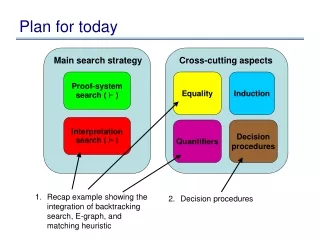
1. Main search strategy Cross-cutting aspects Proof-system search ( ` ) Equality Induction Interpretation search (² ) Quantifiers Decision procedures Plan for today 1. Recap example showing the integration of backtracking search, E-graph, and matching heuristic • Decision procedures

2. Plan for rest of the quarter • Topics still left: • Search in the proof domain: 2 lectures • Equality part II (rewrite systems): 1 lecture • Constructive logic: 1 lecture • Automating induction: 1 lecture

3. A recap example define fact hasConstValue(X:Var,C:Const) with meaning «X == C¬ if currStmt == [X = C] then hasConstValue(X,C)@out if hasConstValue(X,C)@inÆ currStmt == [Y = X] then mustPointTo(Y,C)@out if hasConstantValue(Y,C)@inÆ currStmt == [X = Y] then transform to [X = C]

4. Show that if statements x := y and x := c are executed in a state where y == c, then the resulting states are the same. VC for the trans rule if hasConstantValue(Y,C)@inÆ currStmt == [X = Y] then transform to [X = C]

5. Show that if statements x := y and x := c are executed in a state where y == c, then the resulting states are the same. • Show: • 8x,y,c, . [y] = c • 8v . step(x := y, )[v] = • step(x := c, )[v] ) VC for the trans rule

6. Show: • 8x,y,c, . [y] = c • 8v . step(x := y, )[v] = • step(x := c, )[v] ) Background axioms • If a := k gets stepped in store , the resulting store is  with “a” updated to “k”. • If a := b gets stepped in store , the resulting store is  with “a” updated to the value of “b”.

7. ` E I ² Q D • Axioms: • 8 a,k, . step(a := k, ) = store(, a, k) • 8a,b, . step(a := b, ) = store(, a, [b]) • Show: • 8x,y,c, . [y] = c • 8v . step(x := y, )[v] = • step(x := c, )[v] ) Background axioms

8. ` E I ² Q D • Axioms: • 8 a,k, . step(a := k, ) = store(, a, k) • 8a,b, . step(a := b, ) = store(, a, [b]) 8x,y,c, . [y] = c 8v . step(x := y, )[v] = step(x := c, )[v] ) Expand • Show:

9. ` E I ² Q D Expand 8x,y,c, . [y] = c 8v . step(x := y, )[v] = step(x := c, )[v] ) : Ç

10. ` E I ² Q D Skolemize 8x,y,c, . [y] = c 8v . step(x := y, )[v] = step(x := c, )[v] : Ç

11. ` E I ² Q D Skolemize : [y] = c Ç step(x := y, )[v] = step(x := c, )[v]

12. ` E I ² Q D Refutation : [y] = c Ç step(x := y, )[v] = step(x := c, )[v] Negate formula and show that the negation is unsatisfiable

13. ` E I ² Q D Refutation [y] = c Æ step(x := y, )[v]  step(x := c, )[v] Negate formula and show that the negation is unsatisfiable

14. ` E I ² Q D Exhaustive interpretation search [y] = c Æ step(x := y, )[v]  step(x := c, )[v] L1 L2

15. ` E I ² Q D Exhaustive interpretation search L1 Æ L1 F T L2 L2 Trivially false F T ? Trivially false

16. ` E I ² Q D L1 ? ? L2 Exhaustive interpretation search Context Search L1 Æ L1 F T L2 L2 Trivially false F T ? Trivially false • Two ways to refute: • Formula becomes trivially false • Set of assumed literals is inconsistent

17. ` E I ² Q D ? ? [y] = c step(x := y, )[v]  step(x := c, )[v] L1, L2, Exhaustive interpretation search Context Search L1 Æ L1 L1 F T L2 L2 L2 F T ?

18. ` E I ² Q D Equality using E-graph [y] = c step(x := y, )[v]  step(x := c, )[v] L1, L2,

19. ` E I ² Q D Equality using E-graph [y] = c step(x := y, )[v]  step(x := c, )[v] [y] c

20. ` E I ² Q D Equality using E-graph [y] = c step(x := y, )[v]  step(x := c, )[v] select step(x := c, ) v [y] c

21. ` E I ² Q D Equality using E-graph [y] = c step(x := y, )[v]  step(x := c, )[v] select select step(x := y, ) step(x := c, ) v [y] c

22. ` E I ² Q D Equality using E-graph [y] = c step(x := y, )[v]  step(x := c, )[v]  select select step(x := y, ) step(x := c, ) v [y] c

23. ` E I ² Q D step(x := c, ) = store(, x, c) Matching 8 a,k, . step(a := k, ) = store(, a, k) • Pick a trigger • If trigger appears in E-graph, instantiate quantifier body  select select step(x := y, ) step(x := c, ) v [y] c

24. ` E I ² Q D Matching 8a,b, . step(a := b, ) = store(, a, [b]) 8 a,k, . step(a := k, ) = store(, a, k) • Pick a trigger • If trigger appears in E-graph, instantiate quantifier body  select select step(x := y, ) step(x := c, ) v [y] c

25. ` E I ² Q D Matching 8a,b, . step(a := b, ) = store(, a, [b]) • Pick a trigger • If trigger appears in E-graph, instantiate quantifier body step(x := y, ) = store(, x, [y])  select select step(x := y, ) step(x := c, ) v [y] c

26. ` E I ² Q D • In summary, add: • step(x := c, ) = store(, x, c) • step(x := y, ) = store(, x, [y])  select select v step(x := y, ) step(x := c, ) Matching [y] c

27. ` E I ² Q D • In summary, add: • step(x := c, ) = store(, x, c) • step(x := y, ) = store(, x, [y])  select select v step(x := y, ) step(x := c, ) [y] c

28. ` E I ² Q D • In summary, add: • step(x := c, ) = store(, x, c) • step(x := y, ) = store(, x, [y])  select select v step(x := y, ) step(x := c, ) store [y] c  x

29. ` E I ² Q D • In summary, add: • step(x := c, ) = store(, x, c) • step(x := y, ) = store(, x, [y])  select select v step(x := y, ) step(x := c, ) store [y] c  x

30. ` E I ² Q D • In summary, add: • step(x := c, ) = store(, x, c) • step(x := y, ) = store(, x, [y])  select select v step(x := y, ) step(x := c, ) store store [y] c  x

31. ` E I ² Q D • In summary, add: • step(x := c, ) = store(, x, c) • step(x := y, ) = store(, x, [y])  select select v step(x := y, ) step(x := c, ) store store [y] c  x

32. ` E I ² Q D Compute congruence closure  select select v step(x := y, ) step(x := c, ) store store [y] c  x

33. ` E I ² Q D ? ? [y] = c step(x := y, )[v]  step(x := c, )[v] L1, L2, Exhaustive Interpretation search Context Search L1 Æ L1 L1 F T L2 L2 L2 F T

34. Decision procedures

35. Decision procedures • Decision procedures are complete algorithms for determining the validity of a formula in a given logic • Decision procedures exist for many logics • EUF • Theory of lists • Theory of arrays • Theory of linear arithmetic over reals or integers • Theory of bit-vectors • …

36. Decision procedures • Decision procedures can be used as standalone provers • But we are more concerned with how decision procedures can be used within the context of a “heuristic” theorem prover • A heuristic theorem prover is a theorem prover for an undecidable logic that uses heuristics to guide its search • We use the term “heuristic” to avoid confusion between the larger heuristic prover and the decision procedures that are being integrated into this larger prover

37. Decision procedures • Why incorporate decision procedures into a heuristic prover? • Because once the search reaches a formula in a decidable subset of the original logic, the strategies of the heuristic prover may be inefficient and incomplete

38. Issues • There are two issues to consider when incorporating decision procedures into a heuristic prover • Communication between decision procedures and the heuristic prover • Communication between decision procedures

39. In Simplify-- • Communication between decision procedures • Don’t have to deal with this, because Simplify-- has only one decision procedure, namely EUF

40. In Simplify-- • Communication form heuristic prover to decision procedures • Communication from decision procedures to the heuristic prover

41. In Simplify-- • Communication form heuristic prover to decision procedures • Push equalities into the E-graph incrementally • Does not require the decision procedure to expose its internal details • Communication from decision procedures to the heuristic prover • Matching heuristic looks into E-graph • Motivation is to improve the heuristic of the prover • For efficiency, expose details of the decision procedure’s data structures • Explicating proofs used to guide the backtracking search • Motivation is efficiency

42. Issues again • Communication between decision procedure and the heuristic prover • We’ve seen how this works in Simplify-- • Communication between decision procedures • This is what’s next

43. Combining decision procedures • Efficient decision procedures exist for many decidable logics, but some formulas do not belong to any of these logics • Instead, they belong to a combination of these logics • For example: if currStmt == [X = Y] then geq(X,Y)@out

44. Nelson-Oppen example • x · y Æ y · x + car(cons(0,x)) Æ P(h(x) – h(y)) Æ: P(0)

45. Nelson-Oppen example • x · y Æ y · x + car(cons(0,x)) Æ P(h(x) – h(y)) Æ: P(0)

46. Correctness • If a contradiction is found, return UNSAT • This is clearly sound, if each decision procedure is sound • If there are no more equalities to be found by any of the decision procedures, return SAT • Is this complete? Have the decision procedures exchanged enough info? • Each decision procedure has found its own satisfying assignments, but how do we know that these satisfying assignments are compatible (ie: don’t contradict each other)

47. Convex theories • A theory is convex if whenever a satisfiable conjunction of literals entails a disjunction of equalities of variables, then it entails one of the equalities • Example: • Theory of linear arithmetic with equalities • For convex theories: • If no equalities can be found, then it is impossible for there to be a disjunction of equalities that can be found; therefore, no missed equalities

48. Nonconvex theories • Example: • Reals under multiplication • xy = 0 Æ z = 0 entails x = z Ç y = z • Integers under + and · • x = 1 Æ y = 2 Æ 1 · z Æ z · 2 entails x = z Ç y = z • Theory of sets • Theory of arrays • For such theories, must perform a case split when a disjunction of equalities is entailed • Try each disjunct recusively. • If any one returns SAT, return SAT • If all disjuncts return UNSAT, return UNSAT

49. Algorithm • Given a formula F that is a conjunction of literals over theories S and T, returns whether F is SAT or UNSAT • Assign conjunctions to FS and FT so that FS is a conjunction of S-literals and FT is a conjunction of T-literals • If either FS or FT is unsatisfiable, return UNSAT • If either FS or FT entails some equality between variables not entailed by the other, then add the equality as a new conjunct to the one that does not entail it. Goto step 2. • If either FS or FT entails a disjunction x1Ç … xk of equalities between variables, then for each i from 1 to k, apply the procedure recursively to FSÆ FTÆ xi. If any recursive call returns SAT, return SAT. Otherwise return UNSAT. • Return SAT

50. Adding Nelson-Oppen to Simplify-- • Each decision procedure keeps track of its own information • Decision procedure for theory T exports a function assert(F), where F is a literal in T • While performing the backtracking search, if a literal is asserted, add that literal (using assert) to the decision procedure for the theory the literal belongs to • If the literal belongs to a combination of theories, split the literal into a conjunction of literals, each one belonging to only one theory