Download
1 / 18
180 likes | 521 Views
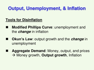
Output, Unemployment, & Inflation. Tools for Disinflation Modified Phillips Curve : unemployment and the change in inflation Okun’s Law : output growth and the change in unemployment Aggregate Demand : Money, output, and prices Money growth, Output growth , Inflation.

E N D
Output, Unemployment, & Inflation Tools for Disinflation • Modified Phillips Curve: unemployment and the change in inflation • Okun’s Law: output growth and the change in unemployment • Aggregate Demand: Money, output, and prices Money growth, Output growth, Inflation
Okun’s Law: The Equation ut - ut-1 = - 0.4 (gyt - 3%) • gyt must be at least 3% to keep unemployment from rising • WHY? • Labor force growth • Increases in labor productivity • Why is the coefficient only 0.4? • Firms need a minimum number of workers • Firms hoard labor • Changes in labor force participation • When economy tanks, workers drop out of the laborforce • u doesn’t rise as much as it otherwise would • Okun’s Law Coefficients Across Countries • Country 1960-1980 1981-1998 • United States 0.39 0.42 United Kingdom 0.15 0.51 Germany* 0.20 0.32 Japan 0.10 0.20
Okun’s Law : how growth in excess of normal growth impacts the unemployment rate : normal growth rate In general, the relation between changes in unem-ployment and output growth is:
The Aggregate Demand Relation: Money Growth (gmt), Inflation (πt), Output Growth (gyt) M/P = Y L(i) Y = (1/L) M/P • Disinflation • According to the AD relation, given inflation, output growth rate decreases when money growth decreases • From Okun’s Law, a decrease in output growth increases unemployment (or reduces it by less than otherwise) • From Modified Phillip’s Curve, • higher unemployment lower inflation
IN MEDIUM RUN: ut = un gy keeps up with productivity and labor force growth and (Assume a constant growth in the nominal money supply) Medium Run: (Okun’s Law) (Aggregate Demand) Output, Unemployment, & Inflation
If decreases to : u remains at un & falls A Adjusted money growth B Adjusted money growth Natural unemployment rate un Output, Unemployment, & Inflation:The Medium Run Adjusting to a decrease in nominal money growth Inflation Rate, Unemployment Rate, u
Disinflation: How much unemployment? And for how long? = Reduce it in 1 yr: Scenario: Reduce inflation from 14 to 4 percent & = 1 Conclusion: Point years of excess unemployment equals 10 The Sacrifice Ratio: Excess point years of unemployment Decrease in Inflation If = 1, what is the sacrifice ratio?
Year Before Disinflation After 0 1 2 3 4 5 6 7 8 Inflation (%) 14 12 10 8 6 4 4 4 4 Δ Inflation 0 -2 -2 -2 -2 -2 0 0 0 Unemployment rate (%) 6.5 8.5 8.5 8.5 8.5 8.5 6.5 6.5 6.5 Output growth (%) 3 -2 3 3 3 3 8 3 3 Nominal money growth (%) 17 10 13 11 9 7 12 7 7 Working on the required path of money growth A Scenario: Reduce inflation from 14% to 4% in 5 years
Year 0 A Year 1 Year 2 Inflation Rate (percent) Year 3 Year 4 Year 5 C B Year 6+ Unemployment Rate (percent) The disinflation path • Transition to lower money growth and inflation is associated with a period of higher unemployment • Regardless of the path, the number of point-years of excess unemployment is the same • In the medium run: output and unemployment return to normal
This model indicates that policy can change the timing but not number of point-years of excess unemployment. • Challenges to this model: Expectations, credibility • Lucas Rat-X New Classical • Sargent Low sacrifice in history Economics Expectations & Credibility: The Lucas Critique • The previous model assumed: te = t-1 • What if teis based on an expectation that Fed policy would reduce inflation from 14% to 4%. • Then: 4% = 4% - 0% • Inflation falls to 4% and unemployment remains at the natural rate • Reduction in money growth could be neutral
A Second Challenge: Nominal rigidities and contractsFischer – sticky wages New Keynesian Taylor – staggered contracts Economics • Disinflation Without Unemployment in the Taylor Model: • Full credibility and staggered wage decisions • Wages in new contracts set close to wages in recent contracts • Commit to slow money growth dramatically in the near future • Wage and price inflation begin to decline when new policy is announced…but only slowly.
The U.S. Disinflation, 1979-1985 1979 • Unemployment = 5.8% • GDP growth = 2.5% • Inflation = 13.3% • The Fed shifted from targeting interest to targeting the growth rate of nominal money
The U.S. Disinflation, 1979-1984 Did Fed credibility reduce the sacrifice ratio? 1979 1980 1981 1982 1983 1984 1985 • GDP growth (%) 2.5 -0.5 1.8 -2.2 3.9 6.2 3.2 • Unemployment rate(%) 5.8 7.1 7.6 9.7 9.6 7.5 7.2 • CPI Inflation (%) 13.3 12.5 8.9 3.8 3.8 3.9 3.8 • Cumulative unemployment 0.6 1.7 4.9 8.0 9.0 9.7 • Cumulative disinflation 0.8 4.4 9.5 9.5 9.4 9.5 • Sacrifice ratio 0.75 0.39 0.51 0.84 0.95 1.02 Cumulative unemployment is the sum of point-years of excess unemployment from 1980 on, assuming a natural rate of 6.5%. Cumulative disinflation is the difference between inflation in a given year and inflation in 1979. The sacrifice ratio is the ratio of cumulative unemployment to cumulative disinflation. • Disinflation was associated with high unemployment • The sacrifice ratio was very close to 1: 10% disinflation with 10 point-years of excess unemployment • The Modified Phillips Curve relation was very robust
Laurence Ball: Disinflation Experiences in 19 OECD Countries • Disinflation leads to higher unemployment • Faster disinflations are associated with small sacrifice ratios (Lucas/Sargent) • Sacrifice ratios are smaller in countries that have shorter wage contracts (Fischer & Taylor)
Problem 9.6 Get πtdown from 12% to 2% by keeping u at 6% • πt = πte – 1 (u – 5%) a) πte = πt-1 how long to disinflate? b) πte = .25 * 2 + .75 * πt-1 how long to disinflate? c) π1e = .25 * 2 + .75 * π0 & π2e = 2 % how long to disinflate?
Problem 9.3 • Δu = - .4 (gy – 3%) • Δπ = - 1 (u – 5%) • gy = gm – π • un = ? • If u = un and π = 8%. Then gy = ? and gm = ? • Get π down from 8% to 4% in one year! • Trace values of π, u, gyand gm