Download
1 / 26
260 likes | 562 Views
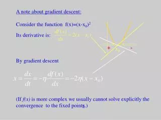
A note about gradient descent: Consider the function f(x)=(x-x 0 ) 2 Its derivative is: By gradient descent (If f(x) is more complex we usually cannot solve explicitly the convergence to the fixed point s .). + -. x 0. Solving the differential equation:.

E N D
A note about gradient descent: Consider the function f(x)=(x-x0)2 Its derivative is: By gradient descent (If f(x) is more complex we usually cannot solve explicitly the convergence to the fixed points.) + - x0
Solving the differential equation: or in the general form: What is the solution of this type of equation: Try:
Objective function formulation We can define a function Rm (Intrator 1992) This function is called a Risk/Objective/Energy/ Lyaponov/Index/Contrast –function in different uses The minimization of this function can be obtained by gradient descent:
Therefore And the stochastic analog is: where It can be shown that the stochastic ODE converges to the deterministic ODE.
Using the objective function formulation: • Fixed points in various cases have been derived. • A connection has been established with the statistical theory of Projection Pursuit • (See chapter 3 of • Theory of Cortical plasticity • Cooper, Intrator, Blais, Shouval )
One way of looking at PCA is that we move to a basis that diagonalizes the correlation matrix. Whereby each PC grows independently. From the basis of the new N principal components xk we can form the rotation matrix such that we get the correlation basis in the new rotated space: so that
What does PCA do? • Dimensionality reduction (hierarchy) • Eliminate correlations – by diagonalizing correlation matrix Graphically: first PC second PC Another thing PCA does is that it finds the projection (direction) of maximal variance. Or assuming |w|=1 and <x>=0
ICA – Independent Component Analysis Usually: Definition of Independent components: In ICA we typically assume this can be done by a linear transformation: Such that x’ are independent. The approach described here follows most closely the work of Hevarinen and Oja (1996,2000)
Cocktail party effect Or in matrix notation Original signals s Mixed signals x s1 x1 s2 x2 Task of ICA – estimate s from x or equivalently estimate the mixing matrix A, or it’s inverse W such that:
Illustration of ICA: s1 s2 x1 0 x2 ( Note the ICA approach only makes sense if the data is indeed a superposition of independent sources)
Definition of independence: This implies that And also implies the private case of decorrelation: But the inverse is not true; decorrelation does not imply independence. Example: pairs of discrete variables (y1,y2) such that points each have the probability of ¼. These variables are uncorrelated, but show at home: 1. that uncorrelated 2. that not independent
Non Gaussian is independent (Caveat – signals cannot be Gaussian) Central limit theorem: “ A sum of many independent random variables approaches a Gaussian distribution as the number of variables increases. Consequently: A sum of two independent, non Gaussian random variables, is “More Gaussian” than each of the signals.
Example Here independent component are sub-Gaussian (light tails) An exponential is super-Gaussian
Contrast functions to measure ‘distance’ from a Gaussian distribution • Kurtosis- a standard simple to understand measure based on the forth moment. • There are two forms of Kurtosis, one is: • typically assume that: E{y}=0 and E{y2}=1, so: At home- calculate the Kurtosis of a uniform distribution form -1 to 1 and an exponential exp(-|x|).
Other options (cost functions): • Negentropy (HO paper 2000) • KL distance between P(x1…xn) and P(x1). …P(xn) (HO paper 2000) • 3. BCM objective function (Theory of … Book 2003- ch 3)
We will use here a similar approach to that used in the objective function formulation of BCM. Use Gradient descent to maximize Kurtosis. What does the sign depend on? However, this rule is not stable for growth of w, and therefore an additional constraint should be used to keep w2=1. This could be done with a similar trick to Oja 1982. For another approach (FastICA see HO, 2000)
Example 1 – cash flow in retail stores Original – preprocessed data 5 Independent components
Example 2: ICA from natural images Are these independent components of natural Images? ICA, BCM and Projection Persuit
Generating Heterosynaptic and Homosynaptic models From Kurtosis we got: This alone is non stable to growth of w. can use the same trick to keep w normalized as in the Oja rule. For this case we obtain: This is a Heterosynaptic rule. Note- the different uses of “Heterosynaptic” Heterosynaptic term
There is another form for Kurtosis: Therefore: This produces a (more complex) Homosynaptic rule with a sliding threshold
General form: Heterosynaptic term What are the consequences of these different rules?
Monocular DeprivationHomosynaptic model (BCM) Low noise High noise
Monocular DeprivationHeterosynaptic model (K2) Low noise High noise
QBCM K1 S1 Noise std Noise std Noise std PCA K2 S2 Noise std Noise std Noise std Noise Dependence of MD Two families of synaptic plasticity rules Homosynaptic Normalized Time Heterosynaptic Normalized Time Blais, Shouval, Cooper. PNAS, 1999