Corner Detection
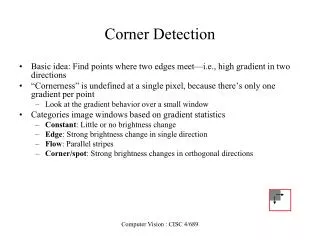
Corner Detection. Basic idea: Find points where two edges meet—i.e., high gradient in two directions “Cornerness” is undefined at a single pixel, because there’s only one gradient per point Look at the gradient behavior over a small window Categories image windows based on gradient statistics

Corner Detection
E N D
Presentation Transcript
Corner Detection • Basic idea: Find points where two edges meet—i.e., high gradient in two directions • “Cornerness” is undefined at a single pixel, because there’s only one gradient per point • Look at the gradient behavior over a small window • Categories image windows based on gradient statistics • Constant: Little or no brightness change • Edge: Strong brightness change in single direction • Flow: Parallel stripes • Corner/spot: Strong brightness changes in orthogonal directions Computer Vision : CISC 4/689
Corner Detection: Analyzing Gradient Covariance • Intuitively, in corner windows both Ix and Iy should be high • Can’t just set a threshold on them directly, because we want rotational invariance • Analyze distribution of gradient components over a window to differentiate between types from previous slide: • The two eigenvectors and eigenvalues ¸1,¸2 of C (Matlab: eig(C)) encode the predominant directions and magnitudes of the gradient, respectively, within the window • Corners are thus where min(¸1, ¸2) is over a threshold courtesy of Wolfram Computer Vision : CISC 4/689
Contents • Harris Corner Detector • Description • Analysis • Detectors • Rotation invariant • Scale invariant • Affine invariant • Descriptors • Rotation invariant • Scale invariant • Affine invariant Computer Vision : CISC 4/689
Window function Shifted intensity Intensity Window function w(x,y) = or 1 in window, 0 outside Gaussian Harris Detector: Mathematics Change of intensity for the shift [u,v]: Computer Vision : CISC 4/689
Harris Detector: Mathematics For small shifts [u,v] we have a bilinear approximation: where M is a 22 matrix computed from image derivatives: Computer Vision : CISC 4/689
Harris Detector: Mathematics Intensity change in shifting window: eigenvalue analysis 1, 2 – eigenvalues of M If we try every possible orientation n, the max. change in intensity is 2 Ellipse E(u,v) = const (max)-1/2 (min)-1/2 Computer Vision : CISC 4/689
Harris Detector: Mathematics 2 Classification of image points using eigenvalues of M: “Edge” 2 >> 1 “Corner”1 and 2 are large,1 ~ 2;E increases in all directions 1 and 2 are small;E is almost constant in all directions “Edge” 1 >> 2 “Flat” region 1 Computer Vision : CISC 4/689
Harris Detector: Mathematics Measure of corner response: (k – empirical constant, k = 0.04-0.06) Computer Vision : CISC 4/689
Harris Detector: Mathematics 2 “Edge” “Corner” • R depends only on eigenvalues of M • R is large for a corner • R is negative with large magnitude for an edge • |R| is small for a flat region R < 0 R > 0 “Flat” “Edge” |R| small R < 0 1 Computer Vision : CISC 4/689
Harris Detector • The Algorithm: • Find points with large corner response function R (R > threshold) • Take the points of local maxima of R Computer Vision : CISC 4/689
Harris Detector: Workflow Computer Vision : CISC 4/689
Harris Detector: Workflow Compute corner response R Computer Vision : CISC 4/689
Harris Detector: Workflow Find points with large corner response: R>threshold Computer Vision : CISC 4/689
Harris Detector: Workflow Take only the points of local maxima of R Computer Vision : CISC 4/689
Harris Detector: Workflow Computer Vision : CISC 4/689
Example: Gradient Covariances Corners are whereboth eigenvalues are big from Forsyth & Ponce Detail of image with gradient covar- iance ellipses for 3 x 3 windows Full image Computer Vision : CISC 4/689
Example: Corner Detection (for camera calibration) Computer Vision : CISC 4/689 courtesy of B. Wilburn
Example: Corner Detection courtesy of S. Smith SUSAN corners Computer Vision : CISC 4/689
Harris Detector: Summary • Average intensity change in direction [u,v] can be expressed as a bilinear form: • Describe a point in terms of eigenvalues of M:measure of corner response • A good (corner) point should have a large intensity change in all directions, i.e. R should be large positive Computer Vision : CISC 4/689
Contents • Harris Corner Detector • Description • Analysis • Detectors • Rotation invariant • Scale invariant • Affine invariant • Descriptors • Rotation invariant • Scale invariant • Affine invariant Computer Vision : CISC 4/689
Tracking: compression of video information • Harris response (uses criss-cross gradients) • Dinosaur tracking (using features) • Dinosaur Motion tracking (using correlation) • Final Tracking (superimposed) Courtesy: (http://www.toulouse.ca/index.php4?/CamTracker/index.php4?/CamTracker/FeatureTracking.html) This figure displays results of feature detection over the dinosaur test sequence with the algorithm set to extract the 6 most "interesting" features at every image frame. It is interesting to note that although no attempt to extract frame-to-frame feature correspondences was made, the algorithm still extracts the same set of features at every frame. This will be useful very much in feature tracking. Computer Vision : CISC 4/689
One More.. • Office sequence • Office Tracking Computer Vision : CISC 4/689
Harris Detector: Some Properties • Rotation invariance Ellipse rotates but its shape (i.e. eigenvalues) remains the same Corner response R is invariant to image rotation Computer Vision : CISC 4/689
Intensity scale: I aI R R threshold x(image coordinate) x(image coordinate) Harris Detector: Some Properties • Partial invariance to affine intensity change • Only derivatives are used => invariance to intensity shift I I+b Computer Vision : CISC 4/689
Harris Detector: Some Properties • But: non-invariant to image scale! All points will be classified as edges Corner ! Computer Vision : CISC 4/689
Harris Detector: Some Properties • Quality of Harris detector for different scale changes -- Correspondences calculated using distance (and threshold) -- Improved Harris is proposed by Schmid et al -- repeatability rate is defined as the number of points repeated between two images w.r.t the total number of detected points. Repeatability rate: # correspondences# possible correspondences Imp.Harris uses derivative of Gaussian instead of standard template used by Harris et al. Computer Vision : CISC 4/689 C.Schmid et.al. “Evaluation of Interest Point Detectors”. IJCV 2000
Contents • Harris Corner Detector • Description • Analysis • Detectors • Rotation invariant • Scale invariant • Affine invariant • Descriptors • Rotation invariant • Scale invariant • Affine invariant Computer Vision : CISC 4/689
We want to: detect the same interest points regardless of image changes Computer Vision : CISC 4/689
Models of Image Change • Geometry • Rotation • Similarity (rotation + uniform scale) • Affine (scale dependent on direction)valid for: orthographic camera, locally planar object • Photometry • Affine intensity change (I aI + b) Computer Vision : CISC 4/689
Contents • Harris Corner Detector • Description • Analysis • Detectors • Rotation invariant • Scale invariant • Affine invariant • Descriptors • Rotation invariant • Scale invariant • Affine invariant Computer Vision : CISC 4/689
Rotation Invariant Detection • Harris Corner Detector Computer Vision : CISC 4/689 C.Schmid et.al. “Evaluation of Interest Point Detectors”. IJCV 2000
Contents • Harris Corner Detector • Description • Analysis • Detectors • Rotation invariant • Scale invariant • Affine invariant • Descriptors • Rotation invariant • Scale invariant • Affine invariant Computer Vision : CISC 4/689
Scale Invariant Detection • Consider regions (e.g. circles) of different sizes around a point • Regions of corresponding sizes (at different scales) will look the same in both images Fine/Low Coarse/High Computer Vision : CISC 4/689
Scale Invariant Detection • The problem: how do we choose corresponding circles independently in each image? Computer Vision : CISC 4/689
scale = 1/2 Image 1 f f Image 2 region size region size Scale Invariant Detection • Solution: • Design a function on the region (circle), which is “scale invariant” (the same for corresponding regions, even if they are at different scales) Example: average intensity. For corresponding regions (even of different sizes) it will be the same. • For a point in one image, we can consider it as a function of region size (circle radius) Computer Vision : CISC 4/689
scale = 1/2 Image 1 f f Image 2 s1 s2 region size/scale region size/scale Scale Invariant Detection • Common approach: Take a local maximum of this function Observation: region size (scale), for which the maximum is achieved, should be invariant to image scale. Important: this scale invariant region size is found in each image independently! Max. is called characteristic scale Computer Vision : CISC 4/689
scale = 1/2 Image 1 f f Image 2 s1 s2 region size/scale region size/scale Characteristic Scale Max. is called characteristic scale • The ratio of the scales, at which the extrema were found for corresponding points in two rescaled images, is equal to the scale factor between the images. • Characteristic Scale: Given a point in an image, compute the function responses for several factors sn The characteristic scale is the local max. of the function (can be more than one). • Easy to look for zero-crossings of 2nd derivative than maxima. Computer Vision : CISC 4/689
f f Good ! bad region size f region size bad region size Scale Invariant Detection • A “good” function for scale detection: has one stable sharp peak • For usual images: a good function would be the one with contrast (sharp local intensity change) Computer Vision : CISC 4/689
Scale Invariant Detection Kernels: • Functions for determining scale (Laplacian) (Difference of Gaussians) where Gaussian Note: both kernels are invariant to scale and rotation Computer Vision : CISC 4/689
Build Scale-Space Pyramid • All scales must be examined to identify scale-invariant features • An efficient function is to compute the Difference of Gaussian (DOG) pyramid (Burt & Adelson, 1983) (or Laplacian) Computer Vision : CISC 4/689
Key point localization • Detect maxima and minima of difference-of-Gaussian in scale space Computer Vision : CISC 4/689
scale Laplacian y x Harris scale • SIFT (Lowe)2Find local maximum of: • Difference of Gaussians in space and scale DoG y x DoG Scale Invariant Detectors • Harris-Laplacian1Find local maximum of: • Harris corner detector in space (image coordinates) • Laplacian in scale 1 K.Mikolajczyk, C.Schmid. “Indexing Based on Scale Invariant Interest Points”. ICCV 20012 D.Lowe. “Distinctive Image Features from Scale-Invariant Keypoints”. Accepted to IJCV 2004 Computer Vision : CISC 4/689
Normal, Gaussian.. A normal distribution in a variate with mean and variance2 is a statistic distribution with probability function Computer Vision : CISC 4/689
Harris-Laplacian • Existing methods search for maxima in the 3D representation of an image (x,y,scale). A feature point represents a local maxima in the surrounding 3D cube and its value is higher than a threshold. • THIS (Harris-Laplacian) method uses Harris function first, then selects points for which Laplacian attains maximum over scales. • First, prepare scale-space representation for the Harris function. At each level, detect interest points as local maxima in the image plane (of that scale) – do this by comparing 8-neighborhood. (different from plain Harris corner detection) • Second, use Laplacian to judge if each of the candidate points found on different levels, if it forms a maximum in the scale direction. (check with n-1 and n+1) Computer Vision : CISC 4/689
Scale Invariant Detectors • Experimental evaluation of detectors w.r.t. scale change Repeatability rate: # correspondences# possible correspondences (points present) Computer Vision : CISC 4/689 K.Mikolajczyk, C.Schmid. “Indexing Based on Scale Invariant Interest Points”. ICCV 2001
Scale Invariant Detection: Summary • Given:two images of the same scene with a large scale difference between them • Goal:find the same interest points independently in each image • Solution: search for maxima of suitable functions in scale and in space (over the image) • Methods: • Harris-Laplacian [Mikolajczyk, Schmid]: maximize Laplacian over scale, Harris’ measure of corner response over the image • SIFT [Lowe]: maximize Difference of Gaussians over scale and space Computer Vision : CISC 4/689
Contents • Harris Corner Detector • Description • Analysis • Detectors • Rotation invariant • Scale invariant • Affine invariant (maybe later) • Descriptors • Rotation invariant • Scale invariant • Affine invariant Computer Vision : CISC 4/689
Affine Invariant Detection • Above we considered:Similarity transform (rotation + uniform scale) • Now we go on to:Affine transform (rotation + non-uniform scale) Computer Vision : CISC 4/689
f points along the ray Affine Invariant Detection • Take a local intensity extremum as initial point • Go along every ray starting from this point and stop when extremum of function f is reached • We will obtain approximately corresponding regions Remark: we search for scale in every direction T.Tuytelaars, L.V.Gool. “Wide Baseline Stereo Matching Based on Local, Affinely Invariant Regions”. BMVC2000. Computer Vision : CISC 4/689
Affine Invariant Detection • Algorithm summary (detection of affine invariant region): • Start from a local intensity extremum point • Go in every direction until the point of extremum of some function f • Curve connecting the points is the region boundary • Compute geometric moments of orders up to 2 for this region • Replace the region with ellipse T.Tuytelaars, L.V.Gool. “Wide Baseline Stereo Matching Based on Local, Affinely Invariant Regions”. BMVC2000. Computer Vision : CISC 4/689