Download
1 / 28
280 likes | 390 Views
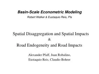
Basin-Scale Econometric Modeling Robert Walker & Eustaquio Reis, PIs. Spatial Disaggregation and Spatial Impacts & Road Endogeneity and Road Impacts Alexander Pfaff, Juan Robalino, Eustaquio Reis, Claudio Bohrer. Acknowledgments Michigan State University Robert Walker, Marcellus Caldas,

E N D
Basin-Scale Econometric Modeling Robert Walker & Eustaquio Reis, PIs Spatial Disaggregation and Spatial Impacts & Road Endogeneity and Road Impacts Alexander Pfaff, Juan Robalino, Eustaquio Reis, Claudio Bohrer
Acknowledgments Michigan State UniversityRobert Walker, Marcellus Caldas, Eugenio Arima, Stephen Aldrich University of FloridaStephen Perz Smithsonian Institution William Laurence, Kate Kirby IPEA – Rio Marcia Pimentel Univ. Federal FluminenseSimone Freitas
Related Past Work at this Scale SPACE Cross-sections on forest levels: for BA, Reis and Pfaff e.g. with early basic results from organized data at a basin level, and certainly others (Laurence, Nepstad, and others) since Role of spatial concentration: for BA, Pfaff on population Spatial disaggregation: for BA, Chomitz & Thomas (rain) TIME/HISTORY Dynamics over time: Kerr et al. for Costa Rica 1963-2000 Past Clearing (effect or proxy): CR, Kerr; BA, Chomitz
Recent Work (Andersen & Reis & Weinhold et al.) CONTRIBUTIONS Further efforts on dynamics: examining change over time, exploiting the existence over time of a range of census data Role of concentrated clearing: useful to apply this to roads Both sides of the cost-benefit: examine the economic gains Technique to counter bias: do projections with choice rule Effort to consider causality: further projections techniques LIMITATION: relatively few and often large census units
Going Further – adding space to time Spatially disaggregate using the units of the 1996 census tracts: • apply over time (e.g., forest in 1976 onward) for dynamics • permits much greater controls for fixed effects and trends • avoids measurement errors from large-scale aggregation Questions of appropriate measurement: • treatment of the size of units within estimation • appropriate normalization of clearing in a unit Exploit the observations to address the endogeneity of roads: • disaggregate evidence on roads, since 1968, and drivers • explicitly identify and ‘correct’ if roads are non-random
Spatial Disaggregation & Spatial Impacts A. Disaggregated Data • forest loss, both amount & pattern • road change, amount within class B. Regression Results • all observations (census tract & aggregate) • low/medium/high clearing & road effects C. Comparing Results • past clearing & measuring forest change • past clearing & weighting observations
Forest Fragmentation • satellite forest data has resolution within census units and the polygons permit the calculation of “pattern”: • various possible statistics have been linked to habitat • important choice of the unit or scale for calculation, including for the challenge of ‘boundary’ polygons • measurement & linkage to other outcomes and drivers funded by a complementary Tinker Foundation project • UFF is leading our efforts to generate these statistics, currently producing early calculations for large areas
Data Set for Regression Analysis • Forest census tracts ( > 10k) laid over satellite data: Diagnostico for earlier years; TRFIC for later years; measuring the probability a forest parcel is cleared • Roads: census tracts laid over maps of the network for 1968, 1975, 1981, 1987, 1993 (four transitions); measuring initial levels and changes in the densities for six classes (using paved, ‘unpaved’ and other) • Census data (larger units): population, PIB changes • Rainfall and Soil Fertility, plus Slopes and Distances
Representative Results(aggregate is similar) ------------------------------------------------- ahz7687 | Coef. Std. Err. t P>|t| ---------+--------------------------------------- rp6875 | .0015357 .0002685 5.72 0.000 rp6875cp | -.0028917 .0008406 -3.44 0.001 ri6875 | .0000117 .0000396 0.29 0.768 ri6875cp | .0047655 .0036552 1.30 0.192 cp76 | .3991804 .0213409 18.70 0.000 pibd7075 | (dropped) popd7075 | (dropped) dtsc | -.0000137 .0000135 -1.02 0.308 dtr | .000151 .0000195 7.75 0.000 fertval | .0240908 .0021346 11.29 0.000 slopear | -.2484458 .0637376 -3.90 0.000 slopemt | -.0341709 .0157253 -2.17 0.030 slopeon | -.0253057 .0078283 -3.23 0.001 rain | -8.70e-06 .0002587 -0.03 0.973
Past Clearing & Road Effects • zero previous clearing roads significance the same • some clearing (0–50%) • paved now less significantly positive • unpaved is a bit significantly positive • high clearing (50–100%) • paved now insignificant (“positive”) • unpaved is now again insignificant
Comparing Results on Road Effects • past clearing & measuring forest change: • we look at the probability a forest parcel is cleared, using as a denominator the forest starting the period • growth of cleared land uses clearing as a denominator, leading the measure to fall automatically with clearing • past clearing & weighting observations: • we weight observations according to (varied !!) area, obtaining coefficients with equal weight on any place • without this, highly cleared urban areas overweighted, e.g. double the weight if simply split one unit into two
Summary • major data disaggregation: histories in spatial detail • novel dynamic regressions (with spatial controls): • many other effects that we would expect to see • roads are significantly positive or insignificant • past clearing does matter, including for road effects: • insignificance of road effects if highly cleared • not negative, though, and ‘on average’ positive
Road Endogeneity & Road Impacts A. Disaggregated Forest Transitions 1968 - 1975 • all observations, summed for AML and states • comparing urban and non-urban tracts subsets B. Regression Results “Explaining” Early Roads • where the initial 1968 roads exist vs. not • 1968-1975 investments in paving vs. not C. Matching – a correction of inferences on roads • for each roads tract match on the probability of a road • yields ‘standardized’ comparison of effects on forest
“Explaining” Existence of 1968 Roads ------------------------------------------------- rexist68 | Coef. Std. Err. z P>|z| --------+---------------------------------------- slopear | -10.56795 6.699832 -1.58 0.115 slopefo | -.3946176 .2253968 -1.75 0.080 slopemt | -.4498239 .2764765 -1.63 0.104 slopeso | .4333935 .0765163 5.66 0.000 pibd7075 | -6.262671 3.962876 -1.58 0.114 popd7075 | .0978918 .0557222 1.76 0.079 dtsc | -.002234 .0002047 -10.91 0.000 ac | .8372658 .164225 5.10 0.000 ro | .0306955 .202829 0.15 0.880 am | .5841266 .1143942 5.11 0.000 ra | 1.035408 .1148644 9.01 0.000 mg | .6036166 .1629609 3.70 0.000 ap | 1.158106 .1817405 6.37 0.000 to | .4893222 .1381163 3.54 0.000
Roads vs. None, clearing rates within class Obs.MeanStd. Dev.Roads?Prob.Class 51 .3009592 .3880428 Yes 0.00 - 3711 .1684215 .3261465 No 0.05 128 .3071752 .3761425 Yes 0.05 - • .2614042 .3806753 No 0.10 102 .2103283 .3067487 Yes 0.10 – 776 .1726304 .3179101 No 0.15 82 .2892852 .3763798 Yes 0.15 - 439 .1986469 .3344542 No 0.20 58 .2998738 .3634768 Yes 0.20 - 184 .191915 .3345288 No 0.25
Compare Un/Matched Samples & Clearing Variable Sample | Treated Control %bias %reduct --------------------+--------------------------------- slopeso Unmatched | .38889 .31578 19.5 Matched | .38889 .37327 4.2 78.6 | pibd7075 Unmatched | .01263 .02359 -6.3 Matched | .01263 .00913 2.0 68.1 | dtsc Unmatched | 210.87 303.42 -57.9 Matched | 210.87 214.33 -2.2 96.3 | am Unmatched | .08647 .16748 -24.5 Matched | .08647 .09047 -1.2 95.1 ------------------------------------------------------ ahz7687 Unmatched | .2795 .1932 Difference .0862 ATT | .2795 .2099 Difference .0695
Overall Summary Major data disaggregation: histories in spatial detail, specifically census tract data over time for forest,road (also biophysical maps) (census data more aggregate) Novel dynamic regressions with many spatial obsv’n. : • many clearing observations helps on net road effect • many matching observations helps on endogeneity