Association analysis
Association analysis. Shaun Purcell Boulder Twin Workshop 2004. Overview. Candidate gene association Haplotypes and linkage disequilibrium Linkage and association Family-based association. What is association?. Categorical traits disease susceptibility genes Continuous traits

Association analysis
E N D
Presentation Transcript
Association analysis Shaun Purcell Boulder Twin Workshop 2004
Overview • Candidate gene association • Haplotypes and linkage disequilibrium • Linkage and association • Family-based association
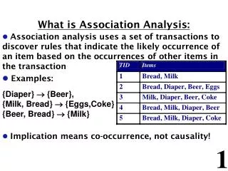
What is association? • Categorical traits • disease susceptibility genes • Continuous traits • quantitative trait loci, QTL
Disease traits Case Control AA n1 n2 Aa n3 n4 aa n5n6 Is there a difference in allele/genotype frequency between cases and controls?
Disease traits Case Control AA 3025 p2 Aa 5050 2p(1-p) aa 20 25 (1-p)2 Is there a difference in allele/genotype frequency between cases and controls? , p-value Test for independence
Disease traits Additive model Dominant model for A General model 1 df 1 df 2 df Effect sizes calculated as odds ratios
Quantitative traits Aa AA aa aa Aa AA ID Y G A D 001 0.34 aa -1 0 002 1.23 Aa 0 1 003 1.66 Aa 0 1 004 2.74 AA 1 0 005 1.33 AA 1 0 … … … … … Y = aA + dD + e
Some web resources • BGIM http://statgen.iop.kcl.ac.uk/bgim/ Introductory tutorials on twin analysis, primer on maximum likelihood, Mx language. • GxE moderator models http://statgen.iop.kcl.ac.uk/gxe/ • Power calculation http://statgen.iop.kcl.ac.uk/gpc/ • Case/control association tools http://statgen.iop.kcl.ac.uk/gpc/model/
Relative risk P(D|AA) / P(D|aa) labelled RR(AA) P(D|Aa) / P(D|aa) labelled RR(Aa)
Multiple samples • Constrain frequencies across samples • Constrain effects across samples • Can test genetic models with effects and/or frequencies constrained to be equal • Can perform tests of homogeneity of effects and/or frequencies across samples
An example2 case/control samples • Population frequency 5%
Homogeneous effects across samples Homogeneous allele frequencies across samples Model p RR(Aa) RR(AA) -2LL ----- - ------ ------ ---- Gen 0.367 1.979 3.663 0.367 1.979 3.663 793.143 Mult 0.367 1.911 3.651 0.367 1.911 3.651 793.199 Dom 0.401 1.990 1.990 0.401 1.990 1.990 802.927 Rec 0.405 1.000 1.921 0.405 1.000 1.921 805.064 None 0.442 1.000 1.000 0.442 1.000 1.000 815.628
Heterogeneous effects across samples Homogeneous allele frequencies across samples Model p RR(Aa) RR(AA) -2LL ----- - ------ ------ ---- Gen 0.367 1.235 2.136 0.367 2.890 5.547 786.498 Mult 0.367 1.440 2.073 0.367 2.282 5.208 788.262 Dom 0.401 1.216 1.216 0.401 2.936 2.936 796.422 Rec 0.405 1.000 1.519 0.405 1.000 2.195 803.849 None 0.443 1.000 1.000 0.443 1.000 1.000 815.628
TESTS OF GENETIC MODELS -- ASSUMING EQ EFFECTS & EQ FREQS ========================================================= Gen vs None (2 df) : 22.485 p = 0.000 Mult vs None (1 df) : 22.429 p = 0.000 Dom vs None (1 df) : 12.701 p = 0.000 Rec vs None (1 df) : 10.564 p = 0.001 Gen vs Mult (1 df) : 0.056 p = 0.813 Gen vs Dom (1 df) : 9.784 p = 0.002 Gen vs Rec (1 df) : 11.921 p = 0.001 TESTS OF GENETIC MODELS -- ASSUMING UNEQ EFFECTS & EQ FREQS =========================================================== Gen vs None (4 df) : 29.130 p = 0.000 Mult vs None (2 df) : 27.366 p = 0.000 Dom vs None (2 df) : 19.205 p = 0.000 Rec vs None (2 df) : 11.779 p = 0.003 Gen vs Mult (2 df) : 1.764 p = 0.414 Gen vs Dom (2 df) : 9.925 p = 0.007 Gen vs Rec (2 df) : 17.351 p = 0.000 TESTS OF EQUAL EFFECTS -- ASSUMING EQ FREQS =========================================== w/ Gen model (2 df) : 6.645 p = 0.036 w/ Mult model (1 df) : 4.938 p = 0.026 w/ Dom model (1 df) : 6.505 p = 0.011 w/ Rec model (1 df) : 1.215 p = 0.270
Indirect association Genotyped markers QTL Ungenotyped markers
Recombination Homologous chromosomes in one parent Paternal chromosome Maternal chromosome Recombination event during meiosis Recombinant gamete transmitted, harboring mutation
Recombination Homologous chromosomes in one parent Paternal chromosome Maternal chromosome No recombination event during meiosis Nonrecombinant gamete transmitted, not harboring mutation
Linkage: affected sib pairs Paternal chromosome Maternal chromosome First affected offspring, no recombination Second affected offspring, recombinant gamete IBD sharing from this one parent (0 or 1) 1 0
Association analysis • Mutation occurs on a ‘red’ chromosome
Association analysis • Mutation occurs on a ‘red’ chromosome
Association analysis • Association due to `linkage disequilibrium’
Haplotypes A a MAM aM mAm am This individual has aa and Mm genotypes and am and aM haplotypes a m M a
Haplotypes A a MAM aM mAm am This individual has Aa and Mm genotypes and AM and am haplotypes … but given only genotype data, consistent with Am/aM as well as AM/am a m A M
Haplotypes A a MAM aM mAm am This individual has AA and Mm genotypes and AM and Am haplotypes A m A M
Equilibrium haplotype frequencies A a Mprpsp mqrqsq r s
Linkage disequilibrium A a Mpr + Dps - Dp mqr - Dqs + Dq r s DMAX = Min(qs, pr) D’ = D /DMAX r2 = D’ / pqrs
Haplotype analysis • Estimate haplotypes from genotypes • Associate haplotypes with trait Haplotype Freq. Odds Ratio AAGG 40% 1.00* AAGT 30% 2.21 CGCG 25% 1.07 AGCT 5% 0.92 * baseline, fixed to 1.00
Linkage Association Sib correlation 0 1 2 IBD at the QTL Trait Trait Sib correlation Sib correlation LD RF aa Aa AA aa Aa AA 0 0 1 1 2 2 QTL genotype Marker genotype IBD at the QTL IBD at the Marker Trait aa Aa AA QTL genotype
Variance Components • Means M1 M2 • Variance-covariance matrix V1 C21 C12 V2 ASSOCIATION LINKAGE
Variance Components • Means M1 +bG1 M2 +bG2 • Variance-covariance matrix V1 C21+q(-½) C12 +q(-½) V2 ASSOCIATION b= regression coef. G = individual’s genotype LINKAGE q= regression coef. = IBD sharing 0 , ½ , 1
Components of a Genetic Theory G G G G G G G G G G G G G G G G G G G G Time G G G G P P • POPULATION MODEL • Allele & genotype frequencies • Demographics & population history • Linkage disequilibrium, haplotype structure • TRANSMISSION MODEL • Mendelian segregation • Identity by descent & genetic relatedness • PHENOTYPE MODEL • Biometrical model of quantitative traits • Additive & dominance components
Linkage without association 3/5 2/6 3/5 2/6 3/6 3/2 5/6 5/2 Both families are ‘linked’ with the marker… …but a different allele is involved.
Linkage and association 3/5 2/6 3/6 2/4 4/6 2/6 3/6 3/2 5/6 6/2 6/6 6/6 All families are ‘linked’ with the marker… … and allele 6 is ‘associated’ with disease Linkage is just association within families
Association without linkage Controls Cases 6/6 6/2 3/5 3/4 3/6 5/6 2/4 3/2 3/6 2/2 4/6 2/6 2/5 5/2 Allele 6 is more common in the GREEN population The disease is more common in the GREEN population … a ‘spurious association’
TDT • Transmission disequilibrium test • test for linkage and association aa Aa AA AA AA Aa Aa AA Aa Aa Aa AA
TDT “A” disease allele AA x Aa AA x Aa aa x Aa aa x Aa AA Aa Aa aa + - + - 0.5 0.5 + - + - 0.5 0.5 Additive Dominant Recessive
Between and within components W B W B W Sib1 = B - W Sib2 = B + W Sib1 Sib2
Between and within components • Fulker et al (1999) Note : W = S1 – B
Parental genotypes • Use parental genotypes to generate B • Examples • AA from AAxAA W = 0 • Aa from AAxAa W = -0.5 • Aa from AaxAa W = 0
assoc.mx • Sibling pair sample • B and W components precalculated in input file • Single SNP genotype • Quantitative trait
assoc.dat s1 s2 g1 g2 b w1 w2 -0.007 -0.972 -1 0 -0.5 -0.5 0.5 -0.829 -0.196 1 1 1 0 0 0.369 0.645 1 1 1 0 0 0.318 1.55 0 1 0.5 -0.5 0.5 1.52 0.910 0 0 0 0 0 -0.948 -1.55 1 1 1 0 0 0.596 -0.394 1 0 0.5 0.5 -0.5 -1.91 -0.905 0 1 0.5 -0.5 0.5 0.499 0.940 1 0 0.5 0.5 -0.5 -1.17 -1.29 1 0 0.5 0.5 -0.5 -0.16 -1.81 1 1 1 0 0
! Mx script for QTL association: sib pairs, univariate Group 1 : Calc NG=2 Begin Matrices; ! ** Parameters B Full 1 1 free ! association : between component W Full 1 1 free ! association : within component M Full 1 1 free ! mean S Full 1 1 free ! Shared residual variance N Full 1 1 free ! Nonshared residual variance ! ** Definition variables ** C Full 1 1 ! association : between X Full 1 1 ! association : within, sib 1 Y Full 1 1 ! association : within, sib 2 End Matrices; ! ** Uncomment for B=W model ! Equate W 1 1 1 B 1 1 1 ! Starting values Matrix B 0 Matrix W 0 Matrix M 0 Matrix S 0.5 Matrix N 0.5 End
Group2 : Data Group Data NI=7 NO=0 RE file=assoc.dat Labels Sib1 Sib2 g1 g2 b w1 w2 Select Sib1 Sib2 b w1 w2 / Definition b w1 w2 / Matrices = Group 1 Means M + B*C + W*X | M + B*C + W*Y / Covariance S + N | S _ S | S + N / Specify C b / Specify X w1 / Specify Y w2 / End
Models B & W B Full 1 1 free W Full 1 1 free !Equate W 1 1 1 B 1 1 1 B = W B Full 1 1 free W Full 1 1 free Equate W 1 1 1 B 1 1 1 B B Full 1 1 free W Full 1 1 !Equate W 1 1 1 B 1 1 1 B=W=0 B Full 1 1 W Full 1 1 !Equate W 1 1 1 B 1 1 1
Tests Test HA H0 Standard association test B = W B=W=0 Test of stratification B & W B = W Robust association test B & W B