Download
1 / 31
310 likes | 342 Views
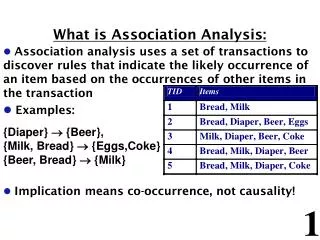
Learn about association analysis, itemsets, candidate generation, support counting, hash trees, subset operations, and rule generation. Understand confidence-based pruning in data mining.

E N D
C1 F1 Itemset Itemset Sup. count {I1} {I1} 6 {I2} {I2} 7 {I3} {I3} 6 {I4} {I4} 2 {I5} {I5} 2 Example Min_sup_count = 2
C2 Itemset {I1,I2} {I1,I3} {I1,I4} {I1,I5} {I2,I3} {I2,I4} {I2,I5} {I3,I4} {I3,I5} {I4,I5} Generate C2 from F1F1 Min_sup_count = 2 F1
Generate C3 from F2F2 Min_sup_count = 2 F2 Prune F3
Generate C4 from F3F3 Min_sup_count = 2 C4 {I1,I2,I3,I5} is pruned because {I2,I3,I5} is infrequent F3
Candidate support counting • Scan the database of transactions to determine the support of each candidate itemset • Brute force: Match each transaction against every candidate. • Too many comparisons! • Better method: Store the candidate itemsets in a hash structure • A transaction will be tested for match only against candidates contained in a few buckets
Generate Hash Tree Hash function 3,6,9 1,4,7 2,5,8 • Suppose you have 15 candidate itemsets of length 3: • {1 4 5}, {1 2 4}, {4 5 7}, {1 2 5}, {4 5 8}, {1 5 9}, {1 3 6}, {2 3 4}, {5 6 7}, {3 4 5}, {3 5 6}, {3 5 7}, {6 8 9}, {3 6 7}, {3 6 8} • You need: • A hash function (e.g. p mod 3) • Max leaf size: max number of itemsets stored in a leaf node (if number of candidate itemsets exceeds max leaf size, split the node) 2 3 4 5 6 7 3 6 7 3 6 8 1 4 5 3 5 6 3 5 7 6 8 9 3 4 5 1 3 6 1 2 4 4 5 7 1 2 5 4 5 8 1 5 9
Hash function 3,6,9 1,4,7 2,5,8 Generate Hash Tree Suppose you have 15 candidate itemsets of length 3: {1 4 5}, {1 2 4}, {4 5 7}, {1 2 5}, {4 5 8}, {1 5 9}, {1 3 6}, {2 3 4}, {5 6 7}, {3 4 5}, {3 5 6}, {3 5 7}, {6 8 9}, {3 6 7}, {3 6 8} 2 3 4 5 6 7 1 4 5 1 3 6 1 2 4 4 5 7 1 2 5 4 5 8 1 5 9 3 5 6 3 5 7 6 8 9 3 4 5 3 6 7 3 6 8 Split nodes with more than 3 candidates using the second item
Hash function 3,6,9 1,4,7 2,5,8 Generate Hash Tree Suppose you have 15 candidate itemsets of length 3: {1 4 5}, {1 2 4}, {4 5 7}, {1 2 5}, {4 5 8}, {1 5 9}, {1 3 6}, {2 3 4}, {5 6 7}, {3 4 5}, {3 5 6}, {3 5 7}, {6 8 9}, {3 6 7}, {3 6 8} 2 3 4 5 6 7 3 5 6 3 5 7 6 8 9 3 4 5 3 6 7 3 6 8 1 4 5 1 3 6 1 2 4 4 5 7 1 2 5 4 5 8 1 5 9 Now split nodes using the third item
Hash function 3,6,9 1,4,7 2,5,8 Generate Hash Tree Suppose you have 15 candidate itemsets of length 3: {1 4 5}, {1 2 4}, {4 5 7}, {1 2 5}, {4 5 8}, {1 5 9}, {1 3 6}, {2 3 4}, {5 6 7}, {3 4 5}, {3 5 6}, {3 5 7}, {6 8 9}, {3 6 7}, {3 6 8} 2 3 4 5 6 7 3 5 6 3 5 7 6 8 9 3 4 5 3 6 7 3 6 8 1 4 5 1 3 6 1 2 4 4 5 7 1 2 5 4 5 8 1 5 9 Now, split this similarly.
Subset Operation Given a (lexicographically ordered) transaction t, say {1,2,3,5,6} how can we enumerate the possible subsets of size 3?
3 + 2 + 1 + 5 6 1 2 3 5 6 3 5 6 2 3 5 6 1 4 5 4 5 8 1 2 5 2 3 4 1 2 4 3 6 7 3 6 8 6 8 9 3 5 7 3 5 6 5 6 7 4 5 7 Subset Operation Using Hash Tree Hash Function transaction 1,4,7 3,6,9 2,5,8 1 3 6 3 4 5 1 5 9
1 5 + 2 + 3 + 1 3 + 1 2 + 1 + 6 5 6 1 2 3 5 6 5 6 3 5 6 3 5 6 2 3 5 6 1 4 5 4 5 8 3 6 8 3 6 7 1 2 4 2 3 4 1 2 5 3 5 6 3 5 7 6 8 9 4 5 7 5 6 7 Subset Operation Using Hash Tree Hash Function transaction 1,4,7 3,6,9 2,5,8 1 3 6 3 4 5 1 5 9
Hash Function 2 + 1 5 + 1 + 3 + 1 3 + 1 2 + 6 3 5 6 5 6 5 6 1 2 3 5 6 2 3 5 6 3 5 6 1,4,7 3,6,9 2,5,8 1 4 5 4 5 8 1 2 4 2 3 4 3 6 8 3 6 7 1 2 5 3 5 7 3 5 6 6 8 9 4 5 7 5 6 7 Subset Operation Using Hash Tree transaction 1 3 6 3 4 5 1 5 9 Match transaction against 7 out of 15 candidates
Rule Generation • An association rule can be extracted by partitioning a frequent itemset Y into two nonempty subsets, X and Y -X, such that XY-X satisfies the confidence threshold. • Each frequent k-itemset, Y, can produce up to 2k-2 association rules • ignoring rules that have empty antecedents or consequents. Example Let Y = {1, 2, 3} be a frequent itemset. Six candidate association rules can be generated from Y: {1, 2} {3}, {1, 3}{2}, {2, 3} {1}, {1}{2, 3}, {2} {1, 3}, {3} {1, 2}. Computing the confidence of an association rule does not require additional scans of the transactions. Consider {1, 2}{3}. The confidence is ({1, 2, 3}) / ({1, 2}) Because {1, 2, 3} is frequent, the antimonotone property of support ensures that {1, 2} must be frequent, too, and we know the supports of frequent itemsets.
Confidence-Based Prunning I Theorem. If a rule XY – X does not satisfy the confidence threshold, then any rule X ’Y – X ’, where X ’ is a subset of X, must not satisfy the confidence threshold as well. Proof. Consider the following two rules: X ’ Y – X ’ and XY – X, where X ’X. The confidence of the rules are (Y ) / (X ’) and (Y ) / (X), respectively. Since X ’ is a subset of X, (X ’) (X). Therefore, the former rule cannot have a higher confidence than the latter rule.
Confidence-Based Prunning II • Observe that: X ’Ximplies thatY – X ’ Y – X X’ X Y
Confidence-Based Prunning III • Initially, all the highconfidence rules that have only one item in the rule consequent are extracted. • These rules are then used to generate new candidate rules. • For example, if • {acd} {b} and {abd} {c} are highconfidence rules, then the candidate rule {ad} {bc} is generated by merging the consequents of both rules.
Confidence-Based Prunning IV {Bread,Milk}{Diaper} (confidence = 3/3)threshold=50% {Bread,Diaper}{Milk} (confidence = 3/3) {Diaper,Milk}{Bread} (confidence = 3/3) Items (1-itemsets) Pairs (2-itemsets) Triplets (3-itemsets)
Confidence-Based Prunning V Merge: {Bread,Milk}{Diaper} {Bread,Diaper}{Milk} {Bread}{Diaper,Milk} (confidence = 3/4) …
Compact Representation of Frequent Itemsets • Some itemsets are redundant because they have identical support as their supersets • Number of frequent itemsets • Need a compact representation
Maximal Frequent Itemsets An itemset is maximal frequent if none of its immediate supersets is frequent Maximal Itemsets Maximal frequent itemsets form the smallest set of itemsets from which all frequent itemsets can be derived. Infrequent Itemsets Border
Maximal Frequent Itemsets • Despite providing a compact representation, maximal frequent itemsets do not contain the support information of their subsets. • For example, the support of the maximal frequent itemsets {a, c, e}, {a, d}, and {b,c,d,e} do not provide any hint about the support of their subsets. • An additional pass over the data set is therefore needed to determine the support counts of the nonmaximal frequent itemsets. • It might be desirable to have a minimal representation of frequent itemsets that preserves the support information. • Such representation is the set of the closed frequent itemsets.
Closed Itemset • An itemset is closed if none of its immediate supersets has the same support as the itemset. • Put another way, an itemset X is not closed if at least one of its immediate supersets has the same support count as X. • An itemset is a closed frequent itemset if it is closed and its support is greater than or equal to minsup.
Lattice Transaction Ids Not supported by any transactions
Maximal vs. Closed Itemsets Closed but not maximal Minimum support = 2 Closed and maximal # Closed = 9 # Maximal = 4
Maximal vs Closed Itemsets All maximal frequent itemsets are closed because none of the maximal frequent itemsets can have the same support count as their immediate supersets.
Deriving Frequent Itemsets From Closed Frequent Itemsets • We can use the closed frequent itemsets to determine the support counts for the nonclosed frequent itemsets. • E.g., consider the frequent itemset {a, d}. Because the itemset is not closed, its support count must be identical to one of its immediate supersets. • The key is to determine which superset among {a, b, d}, {a, c, d}, or {a, d, e} has exactly the same support count as {a, d}. • The Apriori principle states that: • Any transaction that contains the superset of {a, d} must also contain {a, d}. • However, any transaction that contains {a, d} does not have to contain the supersets of {a, d}. • So, the support for {a, d} must be equal to the largest support among its supersets. • Since {a, c, d} has a larger support than both {a, b, d} and {a, d, e}, the support for {a, d} must be identical to the support for {a, c, d}.
Support counting using closed frequent itemsets Let C denote the set of closed frequent itemsets Let kmax denote the maximum length of closed frequent itemsets Fkmax ={f | fC, | f | = kmax } {Find all frequent itemsets of size kmax} fork = kmax – 1 downto 1 do Set Fk to be all sub-itemsets of length k from the frequent itemsets in Fk+1 for eachfFkdo iffCthen f.support = max{f’.support | f’Fk+1, f f’} end if end for end for
Computing Frequent Closed Itemsets • We can imagine a set of equivalence classes over the lattice of itemsets: • two itemsets belong to the same equivalence class if they are supported by the same set of transactions. • A closed itemset is also the maximal itemset of an equivalence class. • Finding all these maximal elements of each equivalence class corresponds to finding all the closed itemsets.
Computing Frequent Closed Itemsets • Some algorithms choose the minimal elements (or key patterns) of each equivalence class as closure generators. • A-CLOSE browses the lattice with an Apriori-like strategy, and finds all the minimal elements of each equivalence class. • Since a k-itemset is a key pattern if and only if no one of its (k−1)-subsets has the same support, minimal elements are discovered with subset checking. • In its second step, A-CLOSE calculates the closure of all the minimal generators previously found. • The maximal elements of each equivalence class are produced as output.