Statistical Approaches to Inverse Problems
Statistical Approaches to Inverse Problems. DIIG seminars on inverse problems Insight and Algorithms Niels Bohr Institute Copenhagen, Denmark 27-29 May 2002 (Revised 13 May 2003) P.B. Stark Department of Statistics University of California Berkeley, CA 94720-3860

Statistical Approaches to Inverse Problems
E N D
Presentation Transcript
Statistical Approaches to Inverse Problems DIIG seminars on inverse problems Insight and Algorithms Niels Bohr InstituteCopenhagen, Denmark27-29 May 2002(Revised 13 May 2003) P.B. Stark Department of Statistics University of California Berkeley, CA 94720-3860 www.stat.berkeley.edu/~stark
Abstract It is useful to distinguish between the intrinsic uncertainty of an inverse problem and the uncertainty of applying any particular technique to “solve” the inverse problem. The intrinsic uncertainty depends crucially on the prior constraints on the unknown (including prior probability distributions in the case of Bayesian analyses), on the forward operator, on the statistics of the observational errors, and on the nature of the properties of the unknown one wishes to estimate. I will try to convey some geometrical intuition for uncertainty, and the relationship between the intrinsic uncertainty of linear inverse problems and the uncertainty of some common techniques applied to them.
References & Acknowledgements Donoho, D.L., 1994. Statistical Estimation and Optimal Recovery, Ann. Stat., 22, 238-270. Donoho, D.L., 1995. Nonlinear solution of linear inverse problems by wavelet-vaguelette decomposition, Appl. Comput. Harm. Anal.,2, 101-126. Evans, S.N. and Stark, P.B., 2002. Inverse Problems as Statistics, Inverse Problems, 18, R1-R43 (in press). Stark, P.B., 1992. Inference in infinite-dimensional inverse problems: Discretization and duality, J. Geophys. Res., 97, 14,055-14,082. Stark, P.B., 1992. Minimax confidence intervals in geomagnetism, Geophys. J. Intl., 108, 329-338. Created using TexPoint by G. Necula, http://raw.cs.berkeley.edu/texpoint
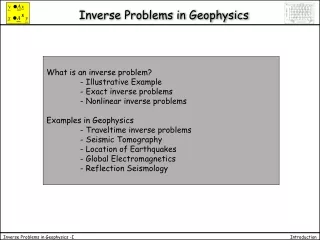
Outline • Inverse Problems as Statistics • Ingredients; Models • Forward and Inverse Problems—applied perspective • Statistical point of view • Some connections • Notation; linear problems; illustration • Example: geomagnetism from satellite observations • Example: seismic velocity from t(p) and x(p) • Example: differential rotation of the Sun from normal mode splitting • Identifiability and uniqueness • Sketch of identifiablity and extremal modeling • Backus-Gilbert theory • Example: solar differential rotation • Example: seismic velocity in Earth’s core
Outline, contd. • Decision Theory • Decision rules and estimators • Comparing decision rules: Loss and Risk • Strategies; Bayes/Minimax duality • Mean distance error and bias • Illustration: Regularization • Illustration: Minimax estimation of linear functionals • Example: Gauss coefficients of the magnetic field • Distinguishing Models: metrics and consistency
Inverse Problems as Statistics • Measurable space X of possible data. • Set of possible descriptions of the world—models. • Family P = {Pq : q2Q} of probability distributions on X, indexed by models . • Forward operatorqaPq maps model into a probability measure on X. Data X are a sample from Pq. Pq is whole story: stochastic variability in the “truth,” contamination by measurement error, systematic error, censoring, etc.
Models • Set usually has special structure. • could be a convex subset of a separable Banach space T. (geomag, seismo, grav, MT, …) • Physical significance of generally gives qaPq reasonable analytic properties, e.g., continuity.
Forward Problems in Geophysics Composition of steps: • transform idealized description of Earth into perfect, noise-free, infinite-dimensional data (“approximate physics”) • censor perfect data to retain only a finite list of numbers, because can only measure, record, and compute with such lists • possibly corrupt the list with measurement error. Equivalent to single-step procedure with corruption on par with physics, and mapping incorporating the censoring.
Inverse Problems Observe data X drawn from distribution Pθ for some unknown . (Assume contains at least two points; otherwise, data superfluous.) Use data X and the knowledge that to learn about ; for example, to estimate a parameter g() (the value g(θ) at θ of a continuous G-valued function g defined on ).
Geophysical Inverse Problems • Inverse problems in geophysics often “solved” using applied math methods for Ill-posed problems (e.g., Tichonov regularization, analytic inversions) • Those methods are designed to answer different questions; can behave poorly with data (e.g., bad bias & variance) • Inference construction: statistical viewpoint more appropriate for interpreting geophysical data.
Elements of the Statistical View Distinguish between characteristics of the problem, and characteristics of methods used to draw inferences. One fundamental property of a parameter: g is identifiable if for all η, z Θ, {g(η) g(z)} {PhPz}. In most inverse problems, g(θ) = θ not identifiable, and few linear functionals of θ are identifiable.
Deterministic and Statistical Connections Identifiability—distinct parameter values yield distinct probability distributions for the observables—similar to uniqueness—forward operator maps at most one model into the observed data. Consistency—parameter can be estimated with arbitrary accuracy as the number of data grows—related to stability of a recovery algorithm—small changes in the data produce small changes in the recovered model. quantitative connections too.
More Notation Let T be a separable Banach space, T* its normed dual. Write the pairing between T and T* <•, •>: T*xTR.
Linear Forward Problems A forward problem is linear if • Θ is a subset of a separable Banach space T • X= Rn, X = (Xj)j=1n • For some fixed sequence (κj)j=1n of elements of T*, Xj = hkj, qi + ej, q2Q, where e = (ej)j=1nis a vector of stochastic errors whose distribution does not depend on θ.
Linear Forward Problems, contd. • Linear functionals {κj} are the “representers” • Distribution Pθ is the probability distribution of X. Typically, dim(Θ) = ; at least, n < dim(Θ), so estimating θ is an underdetermined problem. Define K : TRn q(<κj, θ>)j=1n . Abbreviate forward problem by X = Kθ + ε, θΘ.
Linear Inverse Problems Use X = Kθ + ε, and the constraint θΘ to estimate or draw inferences about g(θ). Probability distribution of X depends on θ only through Kθ, so if there are two points θ1, θ2Θ such that Kθ1 = Kθ2 but g(θ1)g(θ2), then g(θ) is not identifiable.
Ex: Sampling w/ systematic and random error • Observe • Xj = f(tj) + rj + ej, j = 1, 2, …, n, • f 2C, a set of smooth of functions on [0, 1] • tj2 [0, 1] • |rj| 1, j=1, 2, … , n • jiid N(0, 1) • Take Q = C£ [-1, 1]n, X = Rn, and q = (f, r1, …, rn). • Then Pq has density • (2p)-n/2 exp{-åj=1n (xj – f(tj)-rj)2}.
Sketch: Identifiability Pz = Ph Pq X = Rn K K X = K g() g(h) g(z) R {Pz = Ph} ; {h = z}, so q not identifiable g cannot be estimated with bounded bias {Pz = Ph} ; {g(h) = g(z)}, so g not identifiable
Backus-Gilbert Theory Let Q = T be a Hilbert space. Let g 2T = T* be a linear parameter. Let {kj}j=1nµT*. Then: g(q) is identifiable iff g = L¢ K for some 1 £ n matrix L. If also E[e] = 0, then L¢ X is unbiased for g. If also e has covariance matrix S = E[eeT], then the MSE of L¢ X is L¢S¢LT.
Sketch: Backus-Gilbert Pq X = Rn K X = K L¢ X R g() = L¢ Kq
Example: Differential solar rotation • Stellar oscillations known since late 1700s. • Sun's oscillation observed in 1960 by Leighton, Noyes, Simon. Explained as trapped acoustic waves by Ulrich, Leibacher, Stein, 1970-1. Source: SOHO-SOI/MDI website • >107 modes predicted. >250,000 identified; 106 soon Formal error bars inflated by 200. Hill et al., 1996. Science272, 1292-1295
Pattern is Superposition of Modes • Like vibrations of a spherical guitar string • 3 “quantum numbers” l, m, n • l and m are spherical surface wavenumbers • n is radial wavenumber Source: GONG website
Waves Trapped in Waveguide • Low l modes sample more deeply • p-modes do not sample core well • Sun essentially opaque to EM; transparent to sound & to neutrinos Source: forgotten!
Spectrum is very Regular • Explanation as modes, plus stellar evolutionary theory, predict details of spectrum • Details confirmed in data by Deubner, 1975 Source: GONG
Oscillations Taste Solar Interior • Frequencies sensitive to material properties • Frequencies sensitive to differential rotation • If Sun were spherically symmetric and did not rotate, frequencies of the 2l+1 modes with the same l and n would be equal • Asphericity and rotation break the degeneracy (Scheiner measured 27d equatorial rotation from sunspots by 1630. Polar ~33d.) • Like ultrasound for the Sun
Linear forward problem for differential rotation Dnlmn = sklmnW(r,q)r dr dq Language change: q is latitude, W is rotation model. Relationship assumes eigenfunctions and radial structure known. Observational errors usually assumed to be zero-mean independent normal random variables with known variances.
Different Modes sample Sun differently Left: raypath for l=100, n=8 and l=2, n=8 p-modesRight: raypath for l=5, n=10 g-mode. g-modes have not been observed l=20 modes. Left: m=20. Middle: m=16. (Doppler velocities) Right: section through eigenfunction of l=20, m=16, n =14. Gough et al., 1996. Science 272, 1281-1283
Linear Combinations of Splitting Kernels Cuts through kernels for rotation:A: l=15, m=8. B: l=28, m=14. C: l=28, m=24.D: two targeted combinations: 0.7R, 60o; 0.82R, 30oThompson et al., 1996. Science272, 1300-1305. Estimated rotation rate as a function of depth at three latitudes.Source: SOHO-SOI/MDI website
Backus-Gilbert++: Necessary conditions Let g be an identifiable real-valued parameter. Suppose θ0Θ, a symmetric convex set Ť T, cR, and ğ: ŤR such that: • θ0 + ŤΘ • For t Ť, g(θ0 + t) = c + ğ(t), and ğ(-t) = -ğ(t) • ğ(a1t1 + a2t2) = a1ğ(t1) + a2ğ(t2), t1, t2 Ť, a1, a2 0, a1+a2 = 1, and • supt Ť | ğ(t)| <. Then 1×n matrix Λ s.t. the restriction of ğ to Ť is the restriction of Λ.K to Ť.
Backus-Gilbert++: Sufficient Conditions Suppose g = (gi)i=1m is an Rm-valued parameter that can be written as the restriction to Θ of Λ.K for some m×n matrix Λ. Then • g is identifiable. • If E[ε] = 0, Λ.X is an unbiased estimator of g. • If, in addition, ε has covariance matrix Σ = E[εεT], the covariance matrix of Λ.X is Λ.Σ.ΛT whatever be Pθ.
Decision Rules A (randomized) decision rule δ: X M1(A) x δx(.), is a measurable mapping from the space X of possible data to the collection M1(A) of probability distributions on a separable metric space A of actions. Anon-randomized decision rule is a randomized decision rule that, to each x X, assigns a unit point mass at some value a = a(x) A.
Why randomized rules? • In some problems, have better behavior. • Allowing randomized rules can make the set of decisions convex (by allowing mixtures of different decisions), which makes the math easier. • If the risk is convex, Rao-Blackwell theorem says that the optimal decision is not randomized. (More on this later.)
Example: randomization natural Coin has chance 1/3 of landing with one side showing; chance 2/3 of the other showing. Don’t know which side is which. Want to decide whether P(heads) = 1/3 or 2/3. Toss coin 10 times. X = #heads. Toss fair coin once. U = #heads. Use data to pick the more likely scenario, but if data don’t help, decide by tossing a fair coin.
Estimators An estimator of a parameter g(θ) is a decision ruled for which the space A of possible actions is the space G of possible parameter values. ĝ=ĝ(X) is common notation for an estimator of g(θ). Usually write non-randomized estimator as a G-valued function of x instead of a M1(G)-valued function.
Comparing Decision Rules • Infinitely many decision rules and estimators. Which one to use? The best one! But what does best mean?
Loss and Risk • 2-player game: Nature v. Statistician. • Nature picks θ from Θ. θ is secret, but statistician knows Θ. • Statistician picks δ from a set D of rules. δ is secret. • Generate data X from Pθ, apply δ. • Statistician pays loss L(θ, δ(X)). L should be dictated by scientific context, but… • Riskis expected loss: r(θ, δ) = EqL(θ, δ(X)) • Good rule d has small risk, but what does small mean?
Strategy Rare that one d has smallest risk 8qQ. • d is admissible if not dominated (if no estimator does at least as well for every q, and better for some q). • Minimaxdecision minimizes rQ(d) ´ supqQr(θ, δ) over dD • Minimax risk is rQ*´ infd2DrQ(δ) • Bayes decisionminimizes rp(d) ´ sQr(q,d)p(dq) over dD for a given priorprobability distributionp on Q. • Bayes risk is rp*´ infd2D rp(d).
Minimax is Bayes for least favorable prior If minimax risk >> Bayes risk, prior π controls the apparent uncertainty of the Bayes estimate. Pretty generally for convex , D, concave-convexlike r,
Common Risk: Mean Distance Error (MDE) Let dG denote the metric on G, and let ĝ be an estimator of g. MDE at θ of ĝ is MDEθ(ĝ, g) = Eq d(ĝ(X), g(θ)). When metric derives from norm, MDE is called mean norm error (MNE). When the norm is Hilbertian, MNE2 is called mean squared error (MSE).
Shrinkage Suppose X » N(q, I) with dim(q) = d ¸ 3. X not admissible for q for squared-error loss (Stein, 1956). Dominated by dS(X) = X(1 – a/(b + ||X||2)) for small a and big b. James-Stein better: dJS(X) = X(1-a/||X||2), for 0 < a· 2(d-2). Better if take positive part of shrinkage factor: dJS+(X) = X(1-a/||X||2)+, for 0 < a· 2(d-2). Not minimax, but close. Implications for Backus-Gilbert estimates of d¸ 3 linear functionals. 9 extensions to other distributions; see Evans & Stark (1996).
Bias When G is a Banach space, can define bias atθofĝ: biasθ(ĝ, g) = Eq [ĝ - g(θ)] (when the expectation is well-defined). • If biasθ(ĝ, g) = 0, say ĝis unbiased atθ (for g). • If ĝ is unbiased at θ for g for every θ, say ĝ is unbiased for g. If such ĝ exists, say g is unbiasedly estimable. • If g is unbiasedly estimablethen g is identifiable.
Example: Bounded Normal Mean Observe X »N (q, 1). Know a prioriq2 [-t, t]. Want to estimate g(q) = q. Let f(¢) be the standard normal density.Let F(¢) be the standard normal cumulative distribution function. Suppose we elect to use squared-error loss: L(q, d) = (q - d)2 r(q, d) = Eq L(q, d(X)) = Eq (q - d(X))2 rQ(d) = supq2Q r(q, d) = supq2Q Eq (q - d(X))2 rQ* = infd2D supq2Q Eq (q - d(X))2
Risk of X for bounded normal mean Consider simple estimator d(X) = X. EX = q, so X is unbiased for q, and q is unbiasedly estimable. r(q, X) = Eq (q – X)2 = Var(X) = 1. Consider Bayesian prior to capture the constraint q2 [-t, t]: • »p = U[-t, t], the uniform distribution on the interval [-t, t]. rp(X) = s-tt r(q, X) p(dq) = s-tt1£ (2t)-1 dq = 1. In this example, frequentist risk of X equals Bayes risk of X for uniform prior p.
X is not the best: Truncation Easy to find an estimator better than X from both frequentist and Bayes perspectives. Truncation estimate dT dT is biased, but has smaller MSE than X, whatever be q2Q. (dT is the constrained maximum likelihood estimate.)
Risk of dT x Pq(X < -t) dT f(x|q) 0 t -t q -t 0 q t
Minimax Estimation of BNM Truncation estimate better than X, but not minimax. Clear that r*¸ min(1, t2): MSE(X) = 1, and rQ(0) = t2. Minimax MSE estimator is a nonlinear shrinkage estimator. Minimax MSE risk is t2/(1+t2).
Bayes estimation of BNM Posterior density of q given x is