
A Note on Dynamic Data Driven Wildfire Modeling
E N D
Presentation Transcript
A Note on Dynamic Data Driven Wildfire Modeling Jan Mandel University of Colorado at Denver Janice L. Coen, Craig C. Douglas, Leopoldo P. Franca, Craig Johns, Robert Kremens, Anatolii Puhalskii, Anthony Vodacek, Wei Zhao ICCS ‘04 June 7, 2004 Krakow, Poland Supported by NSF under grants ACI-0325314, ACI-0324989, ACI-0324988, ACI-0324876, and ACI-0324910
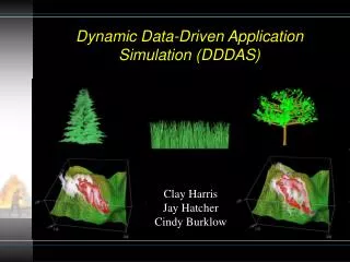
Dynamic Data Driven Application System: Wildfire Weather data Weather model Map sources (GIS) Dynamic Data Assimilation Aerial photos, fuel Fire model Sensors, telemetry Visualization Communication Supercomputing Software engineering
3-dim., time dependent Nonhydrostatic, anelastic Terrain-following coordinates, vertically stretched grid 2-way interacting nested domains Coarse grain parallelization Coupled with an Empirical fire model (based on BEHAVE) Large-scale initialization of atmospheric environment using RUC, MM5, ETA, etc. Models formation of clouds, rain, and hail in “pyrocumulus” clouds over fires Short and long wave atmospheric radiation options Tracks “smoke” dispersion Aspect-dependent solar heating Clark-Hall Atmospheric Model Solve prognostic fluid dynamics equations of motion for air momentum, a thermodynamic variable, water vapor and precipitation on a finite difference grid.
Domain 6 6.7 km 6.7 km Example: Experimental set-up • 6 nested domains: • 10 km, 3.3 km, 1.1 km, 367 m, 122 m, 41 m atm. grid spacing. (Fuel grids can be much finer.). Timestep in finest domain < 1 sec. Inputs Atmosphere • Initialize atmosphere & provide later BCs with MM5 forecast Topography • US 3 sec topography Fuel - Surface and canopy fuels. Loading & Physical characteristics assoc. with Fuel Model. Fuel moisture.
Big Elk Fire SimulationPinewood Springs, CO 17 July 2002 N Red: 10 oC buoyancy White: smoke Frame each 30 sec. W
A Stochastic Reaction-Diffusion Equation Fire Model • Strike a balance between too simple and too slow • Fuel is consumed and generates heat • Heat diffuses, is carried by wind, and radiates into the atmosphere • Embers are carried randomly into distance, cause a local rise of temperature and ignition
N RT 63 RT 20 Max Elevation 5,215’ Max Grade 20% Average Grade 12% Spatial Data Sources for the Model • Base map sources • Aerial photos (Nat’l High Alt.) • SRTM (terrain) • Digital orthoquads • Satellite (Landsat, QuickBird) • WASP (color camera) • Fuels (AVHRR, GAP) • Data sources • Fire (GeoMAC/WASP/others) • Terrain (Shuttle Radar Topographic Mission, SRTM) • RAWS and other Met data • AEDs (Temperature, winds, humidity, radiation, etc. Autonomous Environmental Detectors) WASP project
Fuel Type National database. Overwrite with finer scale where available.
D. McKeown B. Kremens M. Richardson Wildfire Airborne Sensor Program (WASP) High Performance Position Measurement System • Color or Color Infrared Camera • 4k x 4k pixel format • 12 bit quantization • High quality Kodak CCD • Position 5 m • Roll/Pitch 0.03 deg • Heading 0.10 deg • Fire Detection Cameras • 640 x 512 pixel format • 14 bit quantization • < 0.05K NEDT
Time Sequence of Fire PropagationAerial Images from a Prescribed Burn
Image Processing Algorithms (AVIRIS Image from Vodacek et al. and Latham 2002, Int. J. Remote Sensing) 589 nm 770 nm/779 nm • Original image content • Pixel location • Spectral data • Algorithms to register to model grid • auto extraction of tie points • affine transform • Reduced image content • Normalized Thermal Index? • (MWIR-LWIR)/(MWIR+LWIR) • Fire location only (model grid) • Derived temperatures? • Derived fuels? • NDVI (like AVHRR)
Autonomous Environmental Detectors (Primarily for local weather) Data logger and thermocouples We have developed a versatile electronic acquisition package ideally suited to field data collection Major Features Reconfigure to rapidly deploy? Position Aware Versatile Data Inputs Voice or Data Radio telemetry Inexpensive Kremens, et al. 2003. Int. J. Wildland Fire
Dynamic Data Assimilation Present Time Reality Prediction error Data acquisition steering Data Continously Updated Time-Space Model Estimation of model state and parameters from data Prediction
Ensemble Filter: Incorporating Data by a Bayesian Update • Model state is a probability distribution represented as an ensemble of simulation states • Data is a probability distribution represented as the measured values plus error bounds (or better error info) • Observation function relates observations data and simulation states Model State (Forecast Ensemble) Updated Model State (Analysis Ensemble) Bayes Theorem Data: Values, Observation Function
Data Exchange and Formats • Unified format for all data exchange • Observations • Ensemble members (simulation states) • Must contain enough information to construct the observation function: observation=function(simulation state) (from the physics, what the observation would have been in the absence of simulation errors) • Data packets: (coordinates, time-stamp, quantity name, scaling, values)
Dynamic Data Assimilation Driver Module • Initialize ensemble • Advance ensemble in time • Get observation function • Get observation data • Adjust ensemble by a Bayesian update Ensemble Filter Module Model Module • Check for new data • Get data • Request data • Initialize • Export state and stop • Import state and restart • Data Acquisition • Weather data • Image data • Sensor data • Model • Weather-fire simulation • Postprocessing
Standard Approach to Data Assimilation by Ensemble Filter • Generate an initial ensemble by a random perturbation of initial conditions • Repeat the analysis cycle: • Advance ensemble states to a target time by solving the model PDEs in time • Inject data with time-stamps equal to the target time: modify ensemble states by a Bayesian update
Standard Approach to Data Assimilation Bayesian update Advance time Advance time Data Simulation time Analysis cycle
Assimilating Out of Sequence Data(if we can store all time-steps) • Generate initial ensemble by a random perturbation of initial conditions • Repeat the analysis cycle: • Clone the ensemble at the initial time and advance the ensembles except the clone to the next time-step • Inject data into all time-steps: modify the ensemble with states at all time-steps as a single big state,by a Bayesian update
Assimilating Out of Sequence Data(if we can store all time-steps) Advance time Advance time Bayesian update Data Simulation time Analysis cycle
Assimilating Out of Sequence Data(re-create time-steps as needed) • Generate initial ensemble by a random perturbation of initial conditions • Repeat the analysis cycle: • Clone the ensemble at the initial time and other times as needed, advance all ensembles except the clones to their target times, which should include the time-stamp(s) of the data • Inject data into all time-steps: modify the ensemble of states for all stored time-steps as a single big state, by the Bayesian update
Assimilating Out of Sequence Data(re-create time-steps as needed) Advance time-step + to data time Bayesian update Advance time Data Data Data Simulation time Analysis cycle
Least Squares Are No Good Here • Probability distributions (also of the solution) are too far from Gaussian • The problem is too nonlinear Probability density Does not burn: 30% probability Burns: 70% probability Ignition temperature Temperature Least squares solution: does not burn
Visualization • Platform independent: • Web, java based • Browsing from anywhere: PDAs, cell phones,… • Map or 3d terrain, flames • Scenario movies • Maps overlaid with various scenarios • Local outcome probabilities (burn or not) • Input of firefighting scenarios
Supercomputing Resources • What resources needed • Multiple simulations (ensemble 50-500) • Multiple time steps (time-space 10-500) • Actual time step 0.5s, f consists of multiple steps • Multiple interactive firefighting scenarios (1-3) • Mesh sizes • Innermost, finest 200 by 200 by 60 • Outermost, coarsest 50 by 50 by 60 • Total grid point approx. innermost times 2 • 12 fields
This is Work in Progress • Existing: • Clark-Hall model with fire • Fire: stochastic-reaction-convection diffusion PDE • In Progress: • Dynamic data assimilation by Ensemble Kalman Filter • Data conversion and formats • Future: • Use Non-Gaussian Ensemble Filter (literature) • Dynamic data assimilation into the atmosphere-fire model • Real data sources • Visualization • Couple fire PDE model with the Clark-Hall atmosphere model • …