Download
1 / 57
580 likes | 719 Views
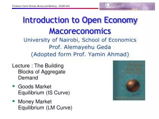
Lecture : The Building Blocks of Aggregate Demand Goods Market Equilibrium (IS Curve) Money Market Equilibrium (LM Curve). Introduction to Open Economy Macoreconomics University of Nairobi, School of Economics Prof. Alemayehu Geda (Adopted form Prof. Yamin Ahmad).

E N D
Lecture : The Building Blocks of Aggregate Demand Goods Market Equilibrium (IS Curve) Money Market Equilibrium (LM Curve) Introduction to Open Economy MacoreconomicsUniversity of Nairobi, School of EconomicsProf. Alemayehu Geda (Adopted form Prof. Yamin Ahmad)
Big Concepts in this lecture… • the IS curve, and its relation to • the Keynesian cross • the loanable funds model • the LM curve, and its relation to • the theory of liquidity preference • how the IS-LM model determines income and the interest rate in the short run when P is fixed Note: These lecture notes are incomplete without having attended lectures
The Big Picture KeynesianCross IScurve IS-LMmodel Explanation of short-run fluctuations Theory of Liquidity Preference LM curve Agg. demandcurve Model of Agg. Demand and Agg. Supply Agg. supplycurve Note: These lecture notes are incomplete without having attended lectures
Context • Second part of lecture 2 introduced the basic model of aggregate demand and aggregate supply. • Long run • prices flexible • output determined by factors of production & technology • unemployment equals its natural rate • Short run • prices fixed • output determined by aggregate demand • unemployment negatively related to output Note: These lecture notes are incomplete without having attended lectures
The Keynesian Cross • A (simpler) closed economy model in which income is determined by expenditure. (due to J.M. Keynes) – book does open economy version of model. • Notation: I = planned investment AE = C + I + G = planned expenditure Y = real GDP = actual expenditure • Difference between actual & planned expenditure = unplanned inventory investment Note: These lecture notes are incomplete without having attended lectures
Elements of the Keynesian Cross Consumption function: Govt policy variables: for now, plannedInvestment is exogenous: planned expenditure: equilibrium condition: actual expenditure = planned expenditure Note: These lecture notes are incomplete without having attended lectures
AE =C +I +G MPC 1 Graphing planned expenditure AE planned expenditure income, output,Y Note: These lecture notes are incomplete without having attended lectures
AE =Y Graphing the equilibrium condition AE planned expenditure 45º income, output,Y Note: These lecture notes are incomplete without having attended lectures
Equilibrium income The equilibrium value of income AE planned expenditure AE =Y AE =C +I +G income, output,Y Note: These lecture notes are incomplete without having attended lectures
AE At Y1, there is now an unplanned drop in inventory… AE =C +I +G2 AE =C +I +G1 G Y AE1 = Y1 AE2 = Y2 Y An increase in government purchases AE =Y …so firms increase output, and income rises toward a new equilibrium. Note: These lecture notes are incomplete without having attended lectures
Solve for Y : Solving for Y equilibrium condition in changes because I exogenous because C= MPCY Collect terms with Yon the left side of the equals sign: Note: These lecture notes are incomplete without having attended lectures
The government purchases multiplier Definition: the increase in income resulting from a $1 increase in G. In this model, the govt purchases multiplier equals Example: If MPC = 0.8, then An increase in G causes income to increase 5 times as much! Note: These lecture notes are incomplete without having attended lectures
Why the multiplier is greater than 1 • Initially, the increase in G causes an equal increase in Y:Y = G. • But Y C furtherY furtherC furtherY • So the final impact on income is much bigger than the initial G. Note: These lecture notes are incomplete without having attended lectures
AE AE =Y AE =C1+I +G AE =C2+I +G At Y1, there is now an unplanned inventory buildup… C = MPC T Y AE2 = Y2 AE1 = Y1 Y An increase in taxes Initially, the tax increase reduces consumption, and therefore E: …so firms reduce output, and income falls toward a new equilibrium Note: These lecture notes are incomplete without having attended lectures
Solving for Y eq’m condition in changes Iand G exogenous Solving for Y : Final result: Note: These lecture notes are incomplete without having attended lectures
The tax multiplier Def: the change in income resulting from a $1 increase in T : If MPC = 0.8, then the tax multiplier equals Note: These lecture notes are incomplete without having attended lectures
The tax multiplier …is negative:A tax increase reduces C, which reduces income. …is greater than one (in absolute value): A change in taxes has a multiplier effect on income. …is smaller than the govt spending multiplier:Consumers save the fraction (1 – MPC) of a tax cut, so the initial boost in spending from a tax cut is smaller than from an equal increase in G. Note: These lecture notes are incomplete without having attended lectures
Walkthrough Example I: Economic Scenario: In the Keynesian Cross, assume that the consumption function is given by: C = 475 + 0.75(Y-T)Planned Investment, I = 150, G = 250, T = 100. • Graph planned expenditure as a function of income • What is the equilibrium level of income • If government purchases increase by 125, what is the new equilibrium income? • What level of government purchases is needed to achieve an income of 2600? Note: These lecture notes are incomplete without having attended lectures
A Balanced Budget Approach Problem: • Suppose that we face our canonical problem where • C=475 + 0.75(Y-T), T = 100 • I = 150, G = 250 • Suppose that the government wishes to increase its spending by 100, but uses a balanced budget approach, thereby raising taxes by the same amount to finance its expenditures. • Question: Is there any impact on GDP? Does it change? If so, by how much? Note: These lecture notes are incomplete without having attended lectures
Balanced Budget Change in G Solution: Suppose G = T=100. Hence i.e. so our balanced budget multiplier = 1 Why? Note: These lecture notes are incomplete without having attended lectures
The IS curve Def: a graph of all combinations of r and Y that result in goods market equilibrium i.e. actual expenditure (output) = planned expenditure The equation for the IS curve is: Note: These lecture notes are incomplete without having attended lectures
AE I Y r Y Deriving the IS curve AE =Y AE =C +I(r2)+G r I AE =C +I(r1)+G AE Y Y1 Y2 r1 r2 IS Y1 Y2 Note: These lecture notes are incomplete without having attended lectures
Why the IS curve is negatively sloped • A fall in the interest rate motivates firms to increase investment spending, which drives up total planned spending (AE). • To restore equilibrium in the goods market, output (a.k.a. actual expenditure, Y) must increase. Note: These lecture notes are incomplete without having attended lectures
Market For Loanable Funds – Closed Economy Define SpY-T-C(Y-T) and Sg T-G S Sp + Sg = Y – C(Y-T) – G = S(Y; G, T) Capital Markets Equilibrium: S(Y;G,T) = I(r)(Loanable Funds) Or Equivalently: Y = Yd C(Y-T) + I(r) + G (+) (+) (-) (+) (-) Note: These lecture notes are incomplete without having attended lectures
r r S2 S1 I(r) Y S, I Y2 Y1 The IScurve and the loanable funds model (a) The L.F. model (b) The IScurve r2 r2 r1 r1 IS Note: These lecture notes are incomplete without having attended lectures
Algebra Of The IS Curve Suppose C = c0 + c1(Y-T) and I = I0 – br (Note: Blanchard also considers the effect of sales on Investment by incorporating Y, i.e. I=b0+b1Y-b2r) Then Y= C + I + G = c0 + I0 + G + c1(Y-T) – br If we collect like terms: Note: These lecture notes are incomplete without having attended lectures
Slope of the IS curve Hold everything except Y and r fixed: Thus IS is relatively flat if either: • b is very large; or • (ii) c close to unity. Note: These lecture notes are incomplete without having attended lectures
Walkthrough Example II: Economic Scenario: Consider the following IS-LM model: Goods Market: C = 200+0.5(Y-T); I = 200 – 1000r; G = 250; T = 200 Question: • Derive the IS relation (i.e. an equation with Y on one side and everything else on the other) Solution Note: These lecture notes are incomplete without having attended lectures
Fiscal Policy and the IS curve • We can use the IS-LM model to see how fiscal policy (G and T) affects aggregate demand and output. • Let’s start by using the Keynesian cross to see how fiscal policy shifts the IS curve… Note: These lecture notes are incomplete without having attended lectures
AE Y r Y Y Shifting the IScurve: G AE =Y AE =C +I(r1)+G2 At any value of r, G AE Y AE =C +I(r1)+G1 …so the IS curve shifts to the right. Y1 Y2 The horizontal distance of the IS shift equals r1 IS2 IS1 Y1 Y2 Note: These lecture notes are incomplete without having attended lectures
Demand for money and demand for bonds! Recall: The Theory of Liquidity Preference • Due to John Maynard Keynes. • A simple theory in which the interest rate is determined by money supply and money demand. • Money supply is exogenous – determined by Fed! • People hold wealth in the form of either: • Money • Bonds Note: These lecture notes are incomplete without having attended lectures
Money supply r interest rate The supply of real money balances is fixed: M/P real money balances Note: These lecture notes are incomplete without having attended lectures
Money demand r interest rate • People either hold: • Money • Bonds • Demand forreal money balances: L(r) M/P real money balances Note: These lecture notes are incomplete without having attended lectures
Equilibrium r interest rate The interest rate adjusts to equate the supply and demand for money: r1 L(r) M/P real money balances Note: These lecture notes are incomplete without having attended lectures
How the Fed raises the interest rate r interest rate To increase r, Fed reduces M r2 r1 L(r) M/P real money balances Note: These lecture notes are incomplete without having attended lectures
CASE STUDY: Monetary Tightening & Interest Rates • Late 1970s: > 10% • Oct 1979: Fed Chairman Paul Volcker announces that monetary policy would aim to reduce inflation • Aug 1979-April 1980: Fed reduces M/P 8.0% • Jan 1983: = 3.7% How do you think this policy change would affect nominal interest rates? Note: These lecture notes are incomplete without having attended lectures
The effects of a monetary tightening on nominal interest rates short run long run model prices prediction actual outcome Monetary Tightening & Rates, cont. Liquidity preference (Keynesian) Quantity theory, Fisher effect (Classical) sticky flexible i > 0 i < 0 8/1979: i= 10.4% 4/1980: i= 15.8% 8/1979: i= 10.4% 1/1983: i= 8.2%
The LM curve Now let’s put Y back into the money demand function: Note: In Blanchard: The LMcurve is a graph of all combinations of r and Y that equate the supply and demand for real money balances. The equation for the LM curve is: Note: These lecture notes are incomplete without having attended lectures
Nominal or Real Rates in Money Demand? What is real return to saving $1? This is known as the Fisher Equation. So: Treat Ms as exogenous; for present set = 0. (-)(+) Note: These lecture notes are incomplete without having attended lectures
r r LM L(r,Y2) L(r,Y1) Y M/P Y1 Y2 Deriving the LM curve (a) The market for real money balances (b) The LM curve r2 r2 r1 r1 Note: These lecture notes are incomplete without having attended lectures
Why the LM curve is upward sloping • An increase in income raises money demand. • Since the supply of real balances is fixed, there is now excess demand in the money market at the initial interest rate. • The interest rate must rise to restore equilibrium in the money market. Note: These lecture notes are incomplete without having attended lectures
Equilibrium in the Bond Market? There are two assets (money and bonds), but only one equilibrium condition. Do we need to worry about bond market equilibrium as well? Answer: No! This is an example of Walras Law. Note: These lecture notes are incomplete without having attended lectures
Algebra of the LM Curve With M and P fixed: 0 = kY - h r Slope of LM Curve : LM curve relatively flat if either: • k small; or • (ii) h large ( “ Liquidity Trap”) Note: These lecture notes are incomplete without having attended lectures
r r LM2 LM1 L(r,Y1) Y M/P Y1 How M shifts the LM curve (a) The market for real money balances (b) The LM curve r2 r2 r1 r1 Note: These lecture notes are incomplete without having attended lectures
Shifts in LM curve (r fixed) • So vertical shift is independent of k Note: These lecture notes are incomplete without having attended lectures
Walkthrough Example III: Economic Scenario: Suppose that the money demand function is: (M/P)d = 1000 – 100rwhere r is the interest rate (in percent). The money supply M is 1000, and the price level is 2. • Graph the supply and demand for real money balances. • What is the equilibrium interest rate? • Assume that the price level is fixed. What happens to the equilibrium interest rate if the supply of money is raised from 1000 to 1200? • If the Fed wishes to raise the interest rate to 7 percent, what money supply should it set? Note: These lecture notes are incomplete without having attended lectures
LM r IS Y The short-run equilibrium The short-run equilibrium is the combination of r and Y that simultaneously satisfies the equilibrium conditions in the goods & money markets: Equilibrium interest rate Equilibrium level of income Note: These lecture notes are incomplete without having attended lectures
Equilibrium With Fixed Prices IS Curve (+)(-)(+) LM Curve (-)(+) Solve for Y and r in terms of G,T, M and P. Note: These lecture notes are incomplete without having attended lectures
r LM Equilibrium interest rate Interest Rate IS Equilibrium level of income Y Income and Output Equilibrium in the IS-LM Model Note: These lecture notes are incomplete without having attended lectures
Is there any reason to expect it to converge to this equilibrium from arbitrary r and Y? • If there is an excess demand for money (excess supply of bonds) this should drive the return on bonds up, and vice versa. • If savings exceeds planned investment, then consumers must be spending less and producers will be accumulating unwanted inventories. So they will cut back production, and vice versa. • Hence the system should converge. Note: These lecture notes are incomplete without having attended lectures