Download
1 / 43
460 likes | 675 Views
Phylogenetics Workhop, 16-18 August 2006. Parsimony and searching tree-space. Barbara Holland. The basic idea. To infer trees we want to find clades (groups) that are supported by synapomorpies (shared derived traits).

E N D
Phylogenetics Workhop, 16-18 August 2006 Parsimony and searching tree-space Barbara Holland
The basic idea • To infer trees we want to find clades (groups) that are supported by synapomorpies (shared derived traits). • More simply put, we assume that if species are similar it is usually due to common descent rather than due to chance.
Sometimes the data agrees ACCGCTTA ACCCCTTA ACTGCTTA Time ACCCCTTA ACCCCATA ACTGCTTA ACTGCTAA ACCCCTTA ACCCCATA ACTGCTTA ACTGCTAA
Sometimes not ACCGCTTA ACTGCTTA ACCCCTTA Time ACCCCTTC ACCCCATA ACTGCTTC ACTGCTAA ACCCCTTC ACCCCATA ACTGCTTC ACTGCTAA
Homoplasy • When we have two or more characters that can’t possibly fit on the same tree without requiring one character to undergo a parallel change or reversal it is called homoplasy. ACCGCTTA ACCCCTTA ACTGCTTA Time ACCCCTTC ACCCCATA ACTGCTTC ACTGCTAA
How can we choose the best tree? • To decide which tree is best we can use an optimality criterion. • Parsimony is one such criterion. • It chooses the tree which requires the fewest mutations to explain the data. • The Principle of Parsimony is the general scientific principle that accepts the simplest of two explanations as preferable.
S1 ACCCCTTC S2 ACCCCATA S3 ACTGCTTC S4 ACTGCTAA (1,2),(3,4) (1,3),(2,4) 1 2 1 3 3 4 2 4
S1 ACCCCTTC S2 ACCCCATA S3 ACTGCTTC S4 ACTGCTAA (1,2),(3,4) 0 (1,3),(2,4) 0 A A A A A A A A
C C T T S1 ACCCCTTC S2 ACCCCATA S3 ACTGCTTC S4 ACTGCTAA (1,2),(3,4) 001 (1,3),(2,4) 002 C C C T C T T T C T
C C G G S1 ACCCCTTC S2 ACCCCATA S3 ACTGCTTC S4 ACTGCTAA (1,2),(3,4) 0011 (1,3),(2,4) 0022 C C C G C G G G C G
A T S1 ACCCCTTC S2 ACCCCATA S3 ACTGCTTC S4 ACTGCTAA (1,2),(3,4) 001101 (1,3),(2,4) 002201 T A T T T A T T A T
A A T T S1 ACCCCTTC S2 ACCCCATA S3 ACTGCTTC S4 ACTGCTAA (1,2),(3,4) 0011011 (1,3),(2,4) 0022011 T T T T T A T A
A C C A S1 ACCCCTTC S2 ACCCCATA S3 ACTGCTTC S4 ACTGCTAA (1,2),(3,4) 00110112 6 (1,3),(2,4) 00220111 7 C A C C C A C A A A According to the parsimony optimality criterion we should prefer the tree (1,2),(3,4) over the tree (1,3),(2,4) as it requires the fewest mutations.
Maximum Parsimony • The parsimony criterion tries to minimise the number of mutations required to explain the data • The “Small Parsimony Problem” is to compute the number of mutations required on a given tree. • For small examples it is straightforward to see how many mutations are needed Cat Cat Rat Rat A G A G G A A A A G G A Dog Dog Mouse Mouse
The Fitch algorithm • For larger examples we need an algorithm to solve the small parsimony problem f Site a A b A c C d C e G f G g T h A g h e a d b c
The Fitch algorithm • Label the tips of the tree with the observed sequence at the site G T A G A C A C
The Fitch algorithm • Pick an arbitrary root to work towards G T A G A C A C
The Fitch algorithm • Work from the tips of the tree towards the root. Label each node with the intersection of the states of its child nodes. • If the intersection is empty label the node with the union and add one to the cost G T A {A,C,G} {A,T} G C A A {C,G} A C A C Cost 4
Fitch continued… • The Fitch algorithm also has a second phase that allocates states to the internal nodes but it does not affect the cost. • To find the Fitch cost of an alignment for a particular tree we just sum the Fitch costs of all the sites.
Tricks to increase efficiency • Ignore constant sites • These must cost 0 on any tree • Ignore parsimony uninformative sites • Unless there are at least two states that occur at least twice the site will have the same score on any tree. • Groups sites with the same pattern • E.g. the site ACCGTA will have the same score as the site CTTAGC as will any site with the pattern wxxyzw
Sankoff algorithm • More general than the Fitch algorithm. • Assumes we have a table of costs cijfor all possible changes between states i and j • For each node k in the tree we compute Sk(i) the minimal cost given that node k is assigned state i. • In particular we can compute the minimum value over i for Sroot(i) which will be the total cost of the character on the tree.
Sankoff algorithm continued • The value of S(i) is easy to compute for the tips of the tree, we assign cost 0 if the observed state is i and otherwise assign cost infinity. • A dynamic programming approach is used to compute the score for an ancestral node a given that the scores of its descendent nodes l and r (left and right) are known.
A G G C T T
Variants • Camin-Sokal parsimony • Two states 0 and 1, change is only possible from state 0 → 1. • Dollo parsimony • A character can evolve only once (0 →1), but can be lost many times (1 → 0) • Ordered states, e.g. 0 → 1 → 2
The “large parsimony problem” • The small parsimony problem – to find the score of a given tree - can be solved in linear time in the size of the tree. • The large parsimony problem is to find the tree with minimum score. • It is known to be NP-Hard.
How many trees are there? An exact search for the best tree, where each tree is evaluated according to some optimality criterion such as parsimony quickly becomes intractable as the number of species increases
Counting trees 1 1 2 3 1 1 1 2 2 3 1 x 3 = 3 3 3 4 4 2 4 1 5 2 1 2 5 1 4 2 1 3 2 5 1 2 1 x 3 x 5 = 15 3 4 3 5 4 5 4 3 3 4
The Chocolate Fish question • First participant to calculate the exact number of unrooted binary trees on 30 taxa collects some fish.
Search strategies • Exact search • possible for small n only • Branch and Bound • up to ~20 taxa • Local Search - Heuristics • pick a good starting tree and use moves within a “neighbourhood” to find a better tree. • Meta-heuristics • Genetic algorithms • Simulated annealing • The ratchet
Exact searches • for small number of taxa (n<=12) it is possible to compute the score of every tree • Branch and Bound searches also guarantee to find the optimal solution but use some clever rules to avoid having to check all trees. They may be effective for up to 25 taxa.
No need to evaluate this whole branch of the search tree, as no tree can have a score better than 9 http://evolution.gs.washington.edu/gs541/2005/lecture25.pdf
Searching tree space • For more than 25 taxa it is usually necessary to use heuristic methods. • When a problem is too hard to solve exactly we use methods that will give a good solution even if we cannot guarantee it will be the best solution. • Start from a good (or perhaps random) tree • Alter the tree using some “move” and check if the new tree has a better score • Keep moving to trees with better scores until no improving move can be found
Moving around in tree-space http://evolution.gs.washington.edu/gs541/2005/lecture25.pdf
Moving around in tree-space optimal http://evolution.gs.washington.edu/gs541/2005/lecture25.pdf
Meta-heuristics • These will sometimes make moves to a tree with a worse score than the current tree. • The advantage is that this makes it possible to avoid becoming trapped in local optima
The ratchet • Randomly reweight the characters • Perform a heuristic search on the altered alignment until a local optima is found • Reset the characters to their original weights • Start a heuristic search beginning from the tree found in step 2 • Repeat steps 1-4 (50-200 times)
Simulated annealing • A random walk through tree space that is biased towards the better scoring trees. • Moves that improve the score are always accepted • Moves the worsen the score may sometimes be accepted depending on • The amount by which the score gets worse • The “temperature” • The temperature is gradually lowered throughout the search • The search can wander widely at first while the temperature is still high but as the temperature is lowered the bias towards making improving moves becomes stronger so it becomes more and more like a pure local search.
Review • Real data sets usually contain homoplasy – characters that do not agree. • To choose the best tree we can use an optimality criterion – this is a way of giving each possible tree a score. • Parsimony is one example of an optimality criterion – it prefers the tree that requires the fewest mutations to explain the data. • In practice we cannot check the score of every tree as there are too many. • Instead we use heuristic searches to explore tree space and find locally optimal trees.