Tree searching
Tree searching. Kai Müller. Tree searching: exhaustive search. branch addition algorithm. Branch and bound. L min =L (random tree) „search tree“ as in branch addition at each level, if L < L min go back one level to try another path


Tree searching
E N D
Presentation Transcript
Tree searching Kai Müller
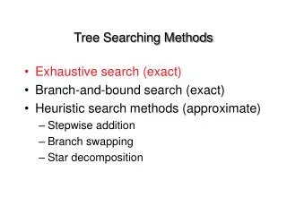
Tree searching: exhaustive search • branch addition algorithm
Branch and bound • Lmin=L(random tree) • „search tree“ as in branch addition • at each level, if L < Lmin go back one level to try another path • if at last level, Lmin=L and go back to first level unless all paths have been tried already
Heuristicsearches best • stepwise addition • as branch addition, but on each level only the path that follows the shortest tree at this level is searched
Branchswapping NNI: nearest neighbour interchanges SPR: subtree pruning and regrafting TBR: tree bisection and reconnection
Tree inference with many terminals • general problem of getting trapped in local optima • searches under parsimony: parsimony ratchet • searches under likelihood: estimation of • substitution model parameters • branch lengths • topology
Parsimonyratchet • generate start tree • TBR on this and the original matrix • perturbe characters by randomly upweighting 5-25%. TBR on best tree found under 2). Go to 2) [200+ times] • once more TBR on current best tree & original matrix • get best trees from those collected in steps 2) and 4)
Bootstrapping • estimates properties of an estimator (such as its variance) by constructing a number of resamples of the observed dataset (and of equal size to the observed dataset), each of which is obtained by random sampling with replacement from the original dataset
Bootstrapping • variants • FWR (Frequencies within replicates) • SC (strict consensus)
Bremer support / decay • Bremer support (decay analysis) is the number of extra steps needed to "collapse" a branch. • searches under reverse constraints: keep trees only that do NOT contain a given node • Takes longer than bootstrapping: parsimony ratchet beneficial (~20 iterations)
Homoplasie-Indices • Consistency Index CI = m/s. • m = die kleinste theoretisch mögliche Schrittzahl die das Merkmal auf einem Baum zeigen könnte • s = Anzahl an tatsächlichen Schritten, die ein Merkmal auf einem gegebenen Baum zeigt • Merkmale ohne Homoplasie haben also einen CI von 1. • Sobald „überschüssige“ Schritte nötig werden, also z.B. s = 3, steigt der Homoplasiegehalt und erniedrigt sich der CI, etwa auf 1/3 = 0.33.
Homoplasie-Indices (2) • Ensemble Consistency Index • Der Ensemble Consistency Index ist dann 1, wenn alle Merkmale nicht homoplastisch sind, also alle perfekt auf den Baum passen. • Nachteile des CI • Parsimonie-uninformative Merkmale tragen immer einen CI von 1 bei und erhöhen so den summarischen CI künstlich. • Andererseits kann der CI nie 0 werden. Gerade das wäre aber eine wünschenswerte Eigenschaft für eine Skala aller denkbaren Homoplasiegrade, die idealerweise von 0 bis 1 reichen sollte. • Drittens wird der CI bei erhöhter Taxonanzahl kleiner, auch wenn sich nichts Wesentliches an dem Informationsgehalt im Datensatz ändert
Homoplasie-Indices (3) • Retention Index (RI) • Wenn g die größtmögliche Schrittzahl eines Merkmals auf jedem denkbaren Baum ist (die auf einem völlig unaufgelösten „Besen“), dann ist RI = (g-s)/(g-m)
Distance methods • observed number vs. actual number of substitutions
Distance methods • observed number vs. actual number of substitutions
Types of substitutions • transitions/transversions • synonymous/non-synonymous
Distance correction correction
Substitution models • p-distance:uncorrected • substitutionmodels • characterizedbysubstitutionprobabilitymatrices:
Substitution models • Jukes-Cantor • oldest (1969), simplest • nucleotide frequencies all identical • nucleotide substitutions all equally likely
P(t) • JC69: • probability of a substitution after time t if mean instant. subst. rate = 10^-8 per site per year
Distances • simple considerations & rearrangements of Pij(t) show that the JC-corrected distance when observing a fraction P of differing nucleotides is
K2P • Kimura 2-parameter model • 2 different nucleotide substitution types • transitions • transversions • nucleotide frequencies all identical
More models • Felsenstein (1981), F81: • 1 nucleotide substitution type, 4 base frequencies • HKY85 • 2 different nucleotide substitution types, 4 base frequencies • GTR • 6 different nucleotide substitution types, 4 base frequencies
Codon models • GY94, MG94 • 61 x 61 matrix (stop codons ignored) = frequency of codon j = transition/transversion ratio = ratio nonsynonymous/synonymous
Models getting more "realistic" • example: covarion models • DNA sites change between „on“ and „off“ states: changes allowed vs. forbidden. • transition rates s01s10, kappa= proportion of „on“:
Additivityofdistances • condition: triangle-inequality • four-point-condition
Correcteddistancesarerarelytree additive! • two approaches try to find the tree that minimizes the error e when fitting the distances on it: • both are tree search-, 2-step methods • least-squares-fit criterion: general: goodness of fit methods • minimum evolution • length L of sum of all branches
Clusteringmethods • 1-step, algorithmic methods • UPGMA • condition of an ultrametrictree
Clustering methods • neighbor joining • star decomposition d(pair members new) node: d(other taxa new node):